Introduction to Linear Functions
For the following exercises, determine whether the equation of the curve can be written as a linear function.
- [latex]y = 3x - 5[/latex]
- [latex]3x + 5y = 15[/latex]
- [latex]3x + 5y^2 = 15[/latex]
- [latex]-\dfrac{x-3}{5} = 2y[/latex]
For the following exercises, determine whether each function is increasing or decreasing.
- [latex]g(x) = 5x + 6[/latex]
- [latex]b(x) = 8 - 3x[/latex]
- [latex]k(x) = -4x + 1[/latex]
- [latex]p(x) = \dfrac{1}{4}x - 5[/latex]
- [latex]m(x) = -\dfrac{3}{8}x + 3[/latex]
For the following exercises, find the slope of the line that passes through the two given points.
- [latex](1,5)[/latex] and [latex](4,11)[/latex]
- [latex](8,-2)[/latex]and [latex](4,6}[/latex]
For the following exercises, which of the tables could represent a linear function? For each that could be linear, find a linear equation that models the data.
-
[latex]x[/latex] [latex]0[/latex] [latex]5[/latex] [latex]10[/latex] [latex]15[/latex] [latex]g(x)[/latex] [latex]5[/latex] [latex]-10[/latex] [latex]-25[/latex] [latex]-40[/latex] -
[latex]x[/latex] [latex]0[/latex] [latex]5[/latex] [latex]10[/latex] [latex]15[/latex] [latex]f(x)[/latex] [latex]-5[/latex] [latex]20[/latex] [latex]45[/latex] [latex]70[/latex] -
[latex]x[/latex] [latex]0[/latex] [latex]2[/latex] [latex]4[/latex] [latex]6[/latex] [latex]g(x)[/latex] [latex]6[/latex] [latex]-19[/latex] [latex]-44[/latex] [latex]-69[/latex] -
[latex]x[/latex] [latex]2[/latex] [latex]4[/latex] [latex]6[/latex] [latex]8[/latex] [latex]f(x)[/latex] [latex]-4[/latex] [latex]16[/latex] [latex]36[/latex] [latex]56[/latex]
Graphs of Linear Functions
For the following exercises, given each set of information, find a linear equation satisfying the conditions, if possible.
- [latex]f(-5) = -4[/latex], and [latex]f(5) = 2[/latex]
- Passes through [latex](2,4)[/latex] and [latex](4,10)[/latex]
- Passes through [latex](-1,4)[/latex] and [latex](5,2)[/latex]
- [latex]x[/latex] intercept at [latex](-2,0)[/latex] and [latex]y[/latex] intercept at [latex](0,-3)[/latex]
For the following exercises, determine whether the lines given by the equations below are parallel, perpendicular, or neither.
- [latex]\begin{align}4x - 7y &= 10 \\ 7x + 4y &= 1\end{align}[/latex]
- [latex]\begin{align}3y + 4x &= 12 \\ -6y = 8x + 1\end{align}[/latex]
For the following exercises, use the descriptions of each pair of lines given below to find the slopes of Line 1 and Line 2. Is each pair of lines parallel, perpendicular, or neither?
- Line 1: Passes through [latex](0,6)[/latex] and [latex](3,-24)[/latex]
Line 2: Passes through [latex](-1,19)[/latex] and [latex](8,-71)[/latex] - Line 1: Passes through [latex](2 ,3 )[/latex] and [latex]( 4,-1 )[/latex]
Line 2: Passes through [latex]( 6,3 )[/latex] and [latex]( 8,5 )[/latex] - Line 1: Passes through [latex]( 2,5 )[/latex] and [latex]( 5,-1 )[/latex]
Line 2: Passes through [latex]( -3,7 )[/latex] and [latex]( 3,-5)[/latex]
For the following exercises, write an equation for the line described.
- Write an equation for a line parallel to [latex]g(x) = 3x - 1[/latex] and passing through the point [latex]( 4,9 )[/latex].
- Write an equation for a line perpendicular to [latex]p(t) = 3t + 4[/latex] and passing through the point [latex]( 3,1 )[/latex].
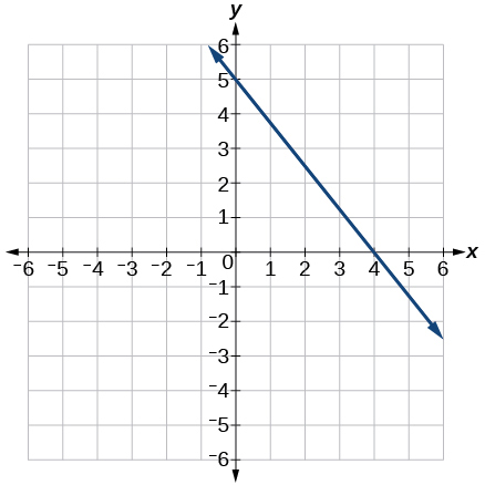
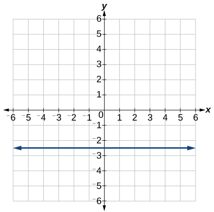
For the following exercises, write an equation for the line graphed.
For the following exercises, match the given linear equation with its graph from the image below.
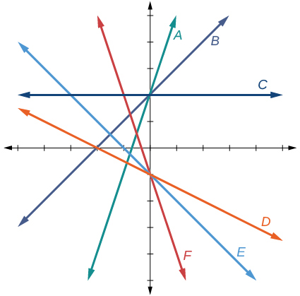
- [latex]f(x) = -3x - 1[/latex]
- [latex]f(x) = 2[/latex]
- [latex]f(x) = 3x + 2[/latex]
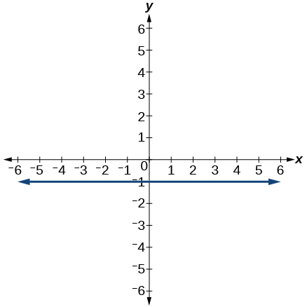
For the following exercises, sketch a line with the given features.
- An [latex]x[/latex]-intercept of [latex](-2,0)[/latex] and [latex]y[/latex]-intercept of [latex](0,4)[/latex]
- A [latex]y[/latex]-intercept of [latex](0,3)[/latex] and slope [latex]\dfrac{2}{5}[/latex]
- Passing through the points [latex](-3,-4)[/latex] and [latex](3,0)[/latex]
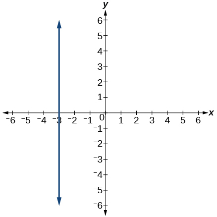
For the following exercises, sketch the graph of each equation.
- [latex]f(x)=-3x+2[/latex]
- [latex]f(x)=\dfrac{2}{3}x-3[/latex]
- [latex]p(t)=-2+3t[/latex]
- [latex]x=-2[/latex]
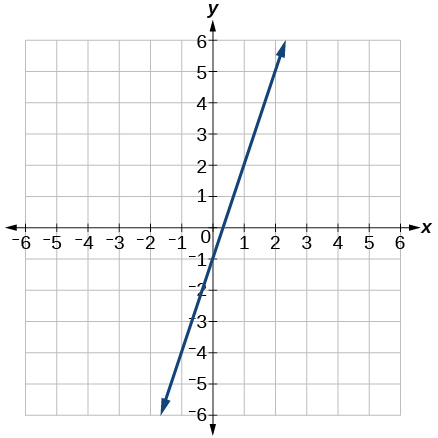
For the following exercises, write the equation of the line shown in the graph.
Fitting Linear Models to Data
For the following exercises, consider this scenario: A town’s population has been decreasing at a constant rate. In 2010 the population was [latex]5,900[/latex]. By 2012 the population had dropped to [latex]4,700[/latex]. Assume this trend continues.
- Predict the population in 2016.
- Identify the year in which the population will reach [latex]0[/latex].
For the following exercises, consider this scenario: A town’s population has been increased at a constant rate. In 2010 the population was [latex]46,020[/latex]. By 2012 the population had increased to [latex]52,070[/latex]. Assume this trend continues.
- Predict the population in 2016.
- Identify the year in which the population will reach [latex]75,000[/latex].
For the following exercises, consider this scenario: A town has an initial population of [latex]75,000[/latex]. It grows at a constant rate of [latex]2,500[/latex] per year for [latex]5[/latex] years.
- Find the linear function that models the town’s population [latex]P[/latex] as a function of the year, [latex]t[/latex], where [latex]t[/latex] is the number of years since the model began.
- Find a reasonable domain and range for the function [latex]P[/latex].
- If the function [latex]P[/latex] is graphed, find and interpret the [latex]x[/latex]– and [latex]y[/latex]-intercepts.
- If the function [latex]P[/latex] is graphed, find and interpret the slope of the function.
- When will the population reach [latex]100,000[/latex]?
- What is the population in the year [latex]12[/latex] years from the onset of the model?
For the following exercises, use the graph below, which shows the profit, [latex]y[/latex], in thousands of dollars, of a company in a given year, [latex]t[/latex], where [latex]t[/latex] represents the number of years since 1980.
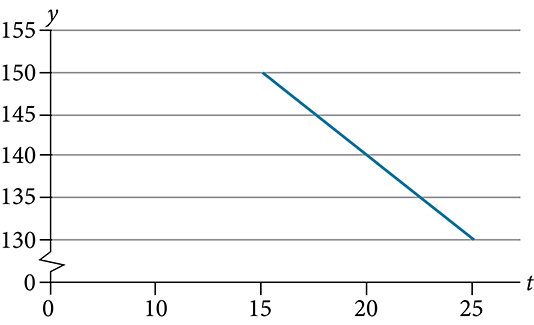
- Find the linear function [latex]y[/latex], where [latex]y[/latex] depends on [latex]t[/latex], the number of years since 1980.
- Find and interpret the [latex]y[/latex]-intercept.
- Find and interpret the [latex]x[/latex]-intercept.
- Find and interpret the slope.
For the following exercises, use the graph below, which shows the profit, [latex]y[/latex], in thousands of dollars, of a company in a given year, [latex]t[/latex], where [latex]t[/latex] represents the number of years since 1980.
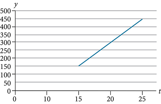
- Find the linear function [latex]y[/latex], where [latex]y[/latex] depends on [latex]t[/latex], the number of years since 1980.
- Find and interpret the [latex]y[/latex]-intercept.
- Find and interpret the [latex]x[/latex]-intercept.
- Find and interpret the slope.
- In 2019, a school population was [latex]1001[/latex]. By 2023 the population had grown to [latex]1697[/latex]. Assume the population is changing linearly.
- How much did the population grow between the year 2019 and 2023?
- How long did it take the population to grow from [latex]1001[/latex] students to [latex]1697[/latex] students?
- What is the average population growth per year?
- What was the population in the year 2015?
- Find an equation for the population, [latex]P[/latex], of the school [latex]t[/latex] years after 2015.
- Using your equation, predict the population of the school in 2026.
- A phone company has a monthly cellular plan where a customer pays a flat monthly fee and then a certain amount of money per minute used for voice or video calling. If a customer uses [latex]410[/latex] minutes, the monthly cost will be [latex]$71.50[/latex]. If the customer uses [latex]720[/latex] minutes, the monthly cost will be [latex]$118[/latex].
- Find a linear equation for the monthly cost of the cell plan as a function of [latex]x[/latex], the number of monthly minutes used.
- Interpret the slope and [latex]y[/latex]-intercept of the equation.
- Use your equation to find the total monthly cost if [latex]687[/latex] minutes are used.
- In 2011, the moose population in a park was measured to be [latex]4,360[/latex]. By 2019, the population was measured again to be [latex]5,880[/latex]. Assume the population continues to change linearly.
- Find a formula for the moose population, [latex]P[/latex] since 2010.
- . What does your model predict the moose population to be in 2023?
- The Federal Helium Reserve held about [latex]16[/latex] billion cubic feet of helium in 2020 and is being depleted by about [latex]2.1[/latex] billion cubic feet each year.
- Give a linear equation for the remaining federal helium reserves, [latex]R[/latex], in terms of [latex]t[/latex], the number of years since 2020.
- In 2025, what will the helium reserves be?
- If the rate of depletion doesn’t change, in what year will the Federal Helium Reserve be depleted?
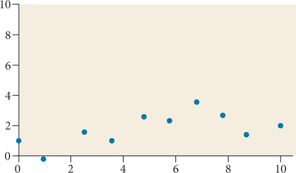
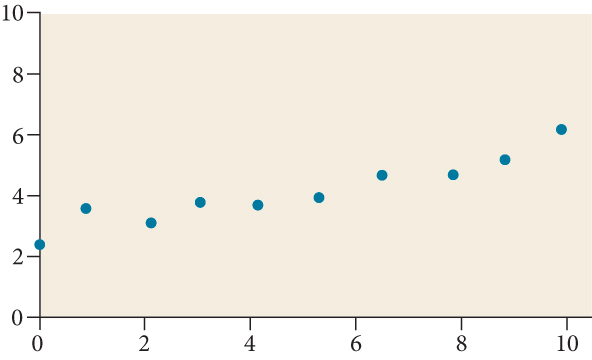
For the following exercises, draw a scatter plot for the data provided. Does the data appear to be linearly related?
-
[latex]1[/latex] [latex]2[/latex] [latex]3[/latex] [latex]4[/latex] [latex]5[/latex] [latex]6[/latex] [latex]46[/latex] [latex]50[/latex] [latex]59[/latex] [latex]75[/latex] [latex]100[/latex] [latex]136[/latex] -
[latex]1[/latex] [latex]3[/latex] [latex]5[/latex] [latex]7[/latex] [latex]9[/latex] [latex]11[/latex] [latex]1[/latex] [latex]9[/latex] [latex]28[/latex] [latex]65[/latex] [latex]125[/latex] [latex]216[/latex] - For the following data, draw a scatter plot. If we wanted to know when the temperature would reach [latex]28^{\circ}\text{F}[/latex], would the answer involve interpolation or extrapolation? Eyeball the line and estimate the answer.
Temperature, [latex]^{\circ}\text{F}[/latex] [latex]16[/latex] [latex]18[/latex] [latex]20[/latex] [latex]25[/latex] [latex]30[/latex] Time, seconds [latex]46[/latex] [latex]50[/latex] [latex]54[/latex] [latex]55[/latex] [latex]62[/latex]
For the following exercises, match each scatterplot with one of the four specified correlations in the figures below.
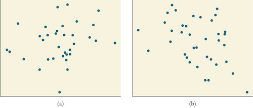
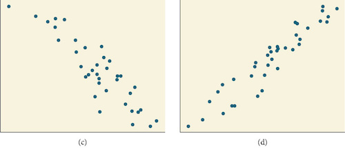
- [latex]r=0.95[/latex]
- [latex]r=-0.89[/latex]
- [latex]r=-0.26[/latex]
- [latex]r=-0.39[/latex]
For the following exercises, draw a best-fit line for the plotted data.
- The U.S. import of wine (in hectoliters) for several years is given in the table below . Determine whether the trend appears linear. If so, and assuming the trend continues, in what year will imports exceed [latex]12,000[/latex] hectoliters?
Year Imports 1992 [latex]2665[/latex] 1994 [latex]2688[/latex] 1996 [latex]3565[/latex] 1998 [latex]4129[/latex] 2000 [latex]4584[/latex] 2002 [latex]5655[/latex] 2004 [latex]6549[/latex] 2006 [latex]7950[/latex] 2008 [latex]8487[/latex] 2009 [latex]9462[/latex]
For the following exercises, use each set of data to calculate the regression line using a calculator or other technology tool, and determine the correlation coefficient to 3 decimal places of accuracy.
-
[latex]x[/latex] [latex]8[/latex] [latex]15[/latex] [latex]26[/latex] [latex]31[/latex] [latex]56[/latex] [latex]y[/latex] [latex]23[/latex] [latex]41[/latex] [latex]53[/latex] [latex]72[/latex] [latex]103[/latex] -
[latex]x[/latex] [latex]3[/latex] [latex]4[/latex] [latex]5[/latex] [latex]6[/latex] [latex]7[/latex] [latex]8[/latex] [latex]9[/latex] [latex]10[/latex] [latex]11[/latex] [latex]12[/latex] [latex]13[/latex] [latex]14[/latex] [latex]15[/latex] [latex]y[/latex] [latex]21.9[/latex] [latex]22.22[/latex] [latex]22.74[/latex] [latex]22.26[/latex] [latex]20.78[/latex] [latex]17.6[/latex] [latex]16.52[/latex] [latex]18.54[/latex] [latex]15.76[/latex] [latex]13.68[/latex] [latex]14.1[/latex] [latex]14.02[/latex] [latex]11.94[/latex] [latex]12.76[/latex] -
[latex]x[/latex] [latex]21[/latex] [latex]25[/latex] [latex]30[/latex] [latex]31[/latex] [latex]40[/latex] [latex]50[/latex] [latex]y[/latex] [latex]17[/latex] [latex]11[/latex] [latex]2[/latex] [latex]-1[/latex] [latex]-18[/latex] [latex]-40[/latex]
For the following exercises, consider this scenario: The population of a city increased steadily over a ten-year span. The following ordered pairs shows the population and the year over the ten-year span, (population, year) for specific recorded years:
[latex](2500,2000), (2650,2001),(3000,2003),(3500,2006),(4200,2010)[/latex]
- Use linear regression to determine a function [latex]y[/latex], where the year depends on the population. Round to three decimal places of accuracy.
- Predict when the population will hit [latex]8,000[/latex].
For the following exercises, consider this scenario: The profit of a company increased steadily over a ten-year span. The following ordered pairs show the number of units sold in hundreds and the profit in thousands of dollars over the ten year span, (number of units sold, profit) for specific recorded years:
[latex](46,250),(48,305),(50,350),(52,390),(54,410)[/latex]
- Use linear regression to determine a function [latex]y[/latex], where the profit in thousands of dollars depends on the number of units sold in hundreds.
- Predict when the profit will exceed one million dollars.
For the following exercises, consider this scenario: The profit of a company decreased steadily over a ten-year span. The following ordered pairs show dollars and the number of units sold in hundreds and the profit in thousands of dollars over the ten-year span (number of units sold, profit) for specific recorded years:
[latex](46,250), (48,225),(50,205),(52,180),(54,165)[/latex]
- Use linear regression to determine a function [latex]y[/latex], where the profit in thousands of dollars depends on the number of units sold in hundreds.
- Predict when the profit will dip below the [latex]$25,000[/latex] threshold.