Graphing Polynomial Functions
Now that we’ve mastered identifying zeros and understanding their multiplicities and behavior, it’s time to bring everything together and graph polynomial functions. Graphing these functions allows us to visualize their behavior and understand the relationships between their algebraic expressions and their graphical representations.
To accurately graph a polynomial function, we’ll consider several key elements:
-
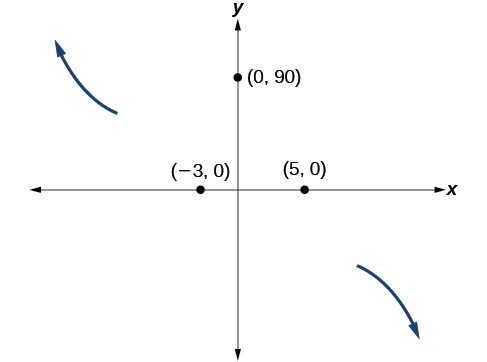
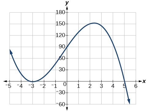
- Zeros and Their Behavior: Where the graph crosses or touches the [latex]x[/latex]-axis.
- For zeros with even multiplicities, the graphs touch or are tangent to the [latex]x[/latex]-axis at these [latex]x[/latex]-values.
- For zeros with odd multiplicities, the graphs cross or intersect the [latex]x[/latex]-axis at these [latex]x[/latex]-values.
- [latex]y[/latex] – intercepts: Points where the graph intersects the [latex]y[/latex]-axis.
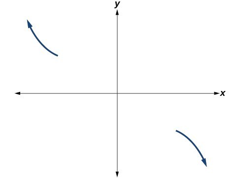
- End Behavior: How the graph behaves as [latex]x[/latex] approaches positive or negative infinity.
- Local Behavior: How the graph behaves near critical points, including turning points and changes in concavity
- Zeros and Their Behavior: Where the graph crosses or touches the [latex]x[/latex]-axis.


- Find the intercepts.
- Check for symmetry. If the function is an even function, its graph is symmetric with respect to the [latex]y[/latex]-axis, that is, [latex]f(–x) = f(x)[/latex].
If a function is an odd function, its graph is symmetric with respect to the origin, that is, [latex]f(–x) = –f(x)[/latex]. - Use the multiplicities of the zeros to determine the behavior of the polynomial at the [latex]x[/latex]-intercepts.
- Determine the end behavior by examining the leading term.
- Use the end behavior and the behavior at the intercepts to sketch the graph.
- Ensure that the number of turning points does not exceed one less than the degree of the polynomial.
- Optionally, use technology to check the graph.
definition
A turning point is a point of the graph where the graph changes from increasing to decreasing (rising to falling) or decreasing to increasing (falling to rising).A polynomial of degree n will have at most n−1 turning points.