Exponential Growth
Because the output of exponential functions increases very rapidly, the term “exponential growth” is often used in everyday language to describe anything that grows or increases rapidly. However, exponential growth can be defined more precisely in a mathematical sense. If the growth rate is proportional to the amount present, the function models exponential growth.
To get a sense of the behavior of exponential growth, we can create a table of values for a function of the form [latex]f(x)={b}^{x}[/latex], where [latex]f \gt 1[/latex].
| [latex]x[/latex] | [latex]–3[/latex] | [latex]–2[/latex] | [latex]–1[/latex] | [latex]0[/latex] | [latex]1[/latex] | [latex]2[/latex] | [latex]3[/latex] |
| [latex]f\left(x\right)={2}^{x}[/latex] | [latex]\frac{1}{8}[/latex] | [latex]\frac{1}{4}[/latex] | [latex]\frac{1}{2}[/latex] | [latex]1[/latex] | [latex]2[/latex] | [latex]4[/latex] | [latex]8[/latex] |
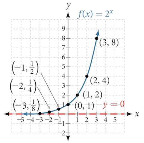
We call the base [latex]2[/latex] the constant ratio. This means that as the input increases by [latex]1[/latex], the output value will be the product of the base and the previous output. Did you notice that the next number is [latex]2[/latex] times the previous number?
This pattern shows exponential growth because the output value increases by a factor of [latex]2[/latex] each time.
Characteristics:
- Domain: [latex](-\infty,\infty)[/latex]
- Range: [latex](0,\infty)[/latex]
- As [latex]x \rightarrow \infty, f(x) \rightarrow \infty[/latex].
- As [latex]x \rightarrow -\infty, f(x) \rightarrow 0[/latex].
- the graph of [latex]f[/latex] will never touch the [latex]x[/latex]-axis because base two raised to any exponent never has the result of zero.
- Horizontal Asymptote: [latex]y = 0[/latex]
- [latex]f(x)[/latex] is always increasing.
- No [latex]x[/latex]-intercept.
- [latex]y[/latex]-intercept is [latex](0,1)[/latex].
exponential growth
A function that models exponential growth grows by a rate proportional to the amount present. For any real number [latex]x[/latex] and any positive real numbers a and b such that [latex]b\ne 1[/latex], an exponential growth function has the form
[latex]\text{ }f\left(x\right)=a{b}^{x}[/latex]
where
- [latex]a[/latex] is the initial or starting value of the function.
- [latex]b[/latex] is the growth factor or growth multiplier per unit [latex]x[/latex].
In more general terms, an exponential function consists of a constant base raised to a variable exponent.
- Company A has [latex]100[/latex] stores and expands by opening [latex]50[/latex] new stores a year, so its growth can be represented by the function [latex]A\left(x\right)=100+50x[/latex].
- Company B has [latex]100[/latex] stores and expands by increasing the number of stores by [latex]50 \%[/latex] each year, so its growth can be represented by the function [latex]B\left(x\right)=100{\left(1+0.5\right)}^{x}[/latex].
A few years of growth for these companies are illustrated below.
| Year, [latex]x[/latex] | Stores, Company A | Stores, Company B |
|---|---|---|
| [latex]0[/latex] | [latex]100 + 50(0) = 100[/latex] | [latex]100(1 + 0.5)^0 = 100[/latex] |
| [latex]1[/latex] | [latex]100 + 50(1) = 150[/latex] | [latex]100(1 + 0.5)^1 = 150[/latex] |
| [latex]2[/latex] | [latex]100 + 50(2) = 200[/latex] | [latex]100(1 + 0.5)^2 = 225[/latex] |
| [latex]3[/latex] | [latex]100 + 50(3) = 250[/latex] | [latex]100(1 + 0.5)^3 = 337.5[/latex] |
| [latex]x[/latex] | [latex]A(x) = 100 + 50x[/latex] | [latex]B(x) = 100(1 + 0.5)^x[/latex] |
The graphs comparing the number of stores for each company over a five-year period are shown below. We can see that, with exponential growth, the number of stores increases much more rapidly than with linear growth.
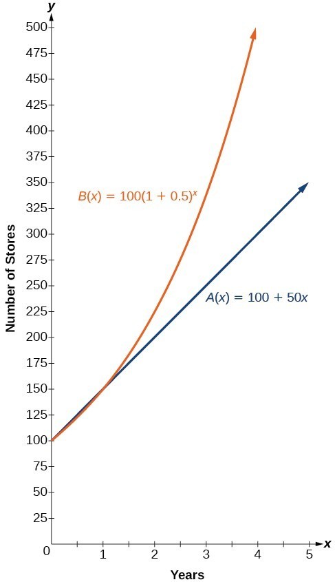
Notice that the domain for both functions is [latex]\left[0,\infty \right)[/latex], and the range for both functions is [latex]\left[100,\infty \right)[/latex]. After year 1, Company B always has more stores than Company A.
Let’s more closely examine the function representing the number of stores for Company B,
In this exponential function, [latex]100[/latex] represents the initial number of stores, [latex]0.5[/latex] represents the growth rate, and [latex]1+0.5=1.5[/latex] represents the growth factor. Generalizing further, we can write this function as
where [latex]100[/latex] is the initial value, [latex]1.5[/latex] is called the base, and [latex]x[/latex] is called the exponent.
[latex]\\[/latex]
This situation is represented by the growth function [latex]P\left(t\right)=1.25{\left(1.012\right)}^{t}[/latex] where [latex]t[/latex] is the number of years since 2013.
[latex]\\[/latex]
To the nearest thousandth, what will the population of India be in 2031?
Exponential Decay
To get a sense of the behavior of exponential decay, we can create a table of values for a function of the form [latex]g(x)={b}^{x}[/latex], where [latex]0 \lt b \lt 1[/latex].
| [latex]x[/latex] | [latex]–3[/latex] | [latex]–2[/latex] | [latex]–1[/latex] | [latex]0[/latex] | [latex]1[/latex] | [latex]2[/latex] | [latex]3[/latex] |
| [latex]g(x)=(\frac{1}{2})^{x}[/latex] | [latex]8[/latex] | [latex]4[/latex] | [latex]2[/latex] | [latex]1[/latex] | [latex]\frac{1}{2}[/latex] | [latex]\frac{1}{4}[/latex] | [latex]\frac{1}{8}[/latex] |
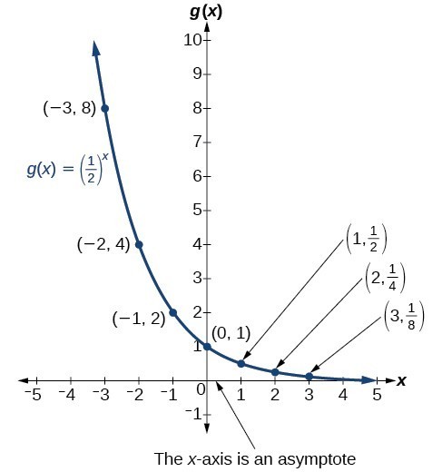
When the input is increasing by [latex]1[/latex], each output value is the product of the previous output and the base or constant ratio [latex]\frac{1}{2}[/latex].
Notice from the table that:
- the output values are positive for all values of [latex]x[/latex].
- as [latex]x[/latex] increases, the output values grow smaller, approaching zero.
- as [latex]x[/latex] decreases, the output values grow without bound.
Characteristics:
- Domain: [latex]\left(-\infty , \infty \right)[/latex]
- Range: [latex]\left(0,\infty \right)[/latex]
- [latex]x[/latex]–intercept: none
- [latex]y[/latex]–intercept: [latex]\left(0,1\right)[/latex]
- Horizontal asymptote: [latex]y=0[/latex]
This is an exponential decay.