Finding a Linear Equation
Building on our understanding of solving equations with a single variable and our introduction to slope, we now turn our attention to linear equations involving two variables. These equations allow us to model relationships between two changing quantities and form the basis for many real-world applications. By exploring the slope-intercept form of linear equations, we’ll connect our algebraic knowledge with graphical representations, providing a powerful tool for analyzing and predicting linear relationships.
Slope-Intercept Form
Perhaps the most familiar form of a linear equation is the slope-intercept form, written as [latex]y=mx+b[/latex], where [latex]m=\text{ slope }[/latex] and [latex]b=y-\text{intercept}[/latex].
slope-intercept form
The slope-intercept form of a line is written as:
[latex]y = mx+b[/latex]
where:
- [latex]m[/latex] is the slope of the line, representing the rate of change or steepness of the line.
- [latex]b[/latex] is the y-intercept, which is the point where the line crosses the y-axis. This value indicates where the line will pass through the y-axis when [latex]x=0[/latex].
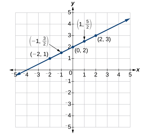
Step 1: Calculate the Slope ([latex]m[/latex])The slope of a line is calculated using the formula [latex]m=\frac{\text{rise}}{\text{run}} = \frac{{y}_{2}-{y}_{1}}{{x}_{2}-{x}_{1}}[/latex].
- Selecting two points from the graph: [latex](-2, 1)[/latex] and [latex](2, 3)[/latex].
- Using these points, we can calculate the slope:
[latex]m = \dfrac{y_2 - y_1}{x_2 - x_1} = \dfrac{3 - 1}{2 - (-2)} = \dfrac{2}{4} = \dfrac{1}{2}[/latex]
Step 2: Find the [latex]y[/latex]-intercept ([latex]b[/latex])
The [latex]y[/latex]-intercept is the value of [latex]y[/latex] when [latex]x=0[/latex]. From the graph, it is apparent that when [latex]x=0, y=2[/latex]. Therefore, [latex]b=2[/latex].
Step 3: Write the Equation
Now that we have the slope and [latex]y[/latex]-intercept, we can write the equation of the line:
[latex]y = \dfrac{1}{2}x+2[/latex]