Stretching, Compressing, or Reflecting an Exponential Function
While horizontal and vertical shifts involve adding constants to the input or to the function itself, a stretch or compression occurs when we multiply the parent function [latex]f\left(x\right)={b}^{x}[/latex] by a constant [latex]|a|>0[/latex].
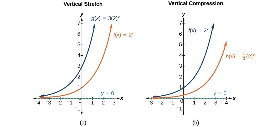
For example, if we begin by graphing the parent function [latex]f\left(x\right)={2}^{x}[/latex], we can then graph the stretch, using [latex]a=3[/latex], to get [latex]g\left(x\right)=3{\left(2\right)}^{x}[/latex] and the compression, using [latex]a=\frac{1}{3}[/latex], to get [latex]h\left(x\right)=\frac{1}{3}{\left(2\right)}^{x}[/latex].
(a) [latex]g\left(x\right)=3{\left(2\right)}^{x}[/latex] stretches the graph of [latex]f\left(x\right)={2}^{x}[/latex] vertically by a factor of 3. (b) [latex]h\left(x\right)=\frac{1}{3}{\left(2\right)}^{x}[/latex] compresses the graph of [latex]f\left(x\right)={2}^{x}[/latex] vertically by a factor of [latex]\frac{1}{3}[/latex].
stretches and compressions of the parent function [latex]f\left(x\right)={b}^{x}[/latex]
The function [latex]f\left(x\right)=a{b}^{x}[/latex]
is stretched vertically by a factor of [latex]a[/latex]if [latex]|a|>1[/latex].
is compressed vertically by a factor of [latex]a[/latex] if [latex]|a|<1[/latex].
has a [latex]y[/latex]-intercept is [latex]\left(0,a\right)[/latex].
has a horizontal asymptote of [latex]y=0[/latex], range of [latex]\left(0,\infty \right)[/latex], and domain of [latex]\left(-\infty ,\infty \right)[/latex] which are all unchanged from the parent function.
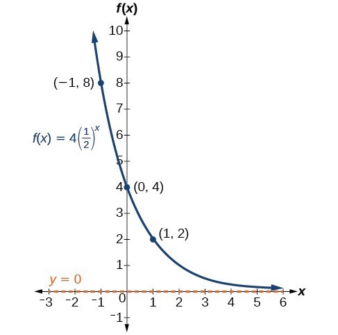
Exponential functions are stretched, compressed or reflected in the same manner you’ve used to transform other functions. Multipliers or negatives inside the function argument (in the exponent) affect horizontal transformations. Multipliers or negatives outside the function argument affect vertical transformations.Sketch a graph of [latex]f\left(x\right)=4{\left(\frac{1}{2}\right)}^{x}[/latex]. State the domain, range, and asymptote.
Before graphing, identify the behavior and key points on the graph.
Since [latex]b=\frac{1}{2}[/latex] is between zero and one, the left tail of the graph will increase without bound as [latex]x[/latex] decreases, and the right tail will approach the [latex]x[/latex]-axis as [latex]x[/latex] increases.
Since [latex]a = 4[/latex], the graph of [latex]f\left(x\right)={\left(\frac{1}{2}\right)}^{x}[/latex] will be stretched vertically by a factor of [latex]4[/latex].
Plot the [latex]y[/latex]–intercept, [latex]\left(0,4\right)[/latex], along with two other points. We can use [latex]\left(-1,8\right)[/latex] and [latex]\left(1,2\right)[/latex].
Draw a smooth curve connecting the points.
The domain is [latex]\left(-\infty ,\infty \right)[/latex], the range is [latex]\left(0,\infty \right)[/latex], the horizontal asymptote is y = 0.
Graphing Reflections
In addition to shifting, compressing, and stretching a graph, we can also reflect it about the [latex]x[/latex]-axis or the [latex]y[/latex]-axis. When we multiply the parent function [latex]f\left(x\right)={b}^{x}[/latex] by [latex]–1[/latex], we get a reflection about the [latex]x[/latex]-axis. When we multiply the input by[latex]–1[/latex], we get a reflection about the [latex]y[/latex]-axis.
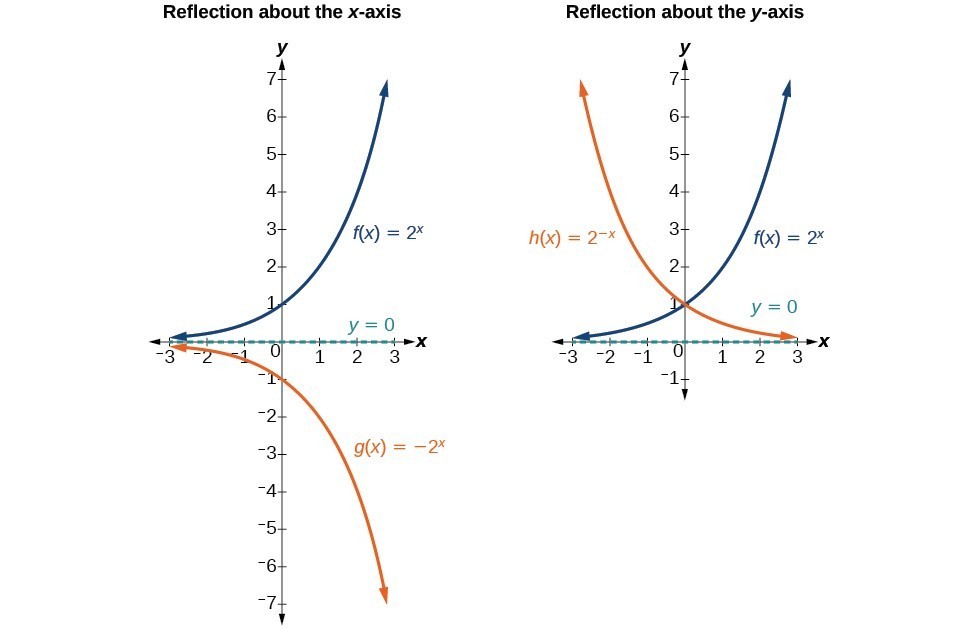
For example, if we begin by graphing the parent function [latex]f\left(x\right)={2}^{x}[/latex], we can then graph the two reflections alongside it. The reflection about the [latex]x[/latex]-axis, [latex]g\left(x\right)={-2}^{x}[/latex], and the reflection about the [latex]y[/latex]-axis, [latex]h\left(x\right)={2}^{-x}[/latex], are both shown below.
(a) [latex]g\left(x\right)=-{2}^{x}[/latex] reflects the graph of [latex]f\left(x\right)={2}^{x}[/latex] about the x-axis. (b) [latex]h\left(x\right)={2}^{-x}[/latex] reflects the graph of [latex]f\left(x\right)={2}^{x}[/latex] about the y-axis.
reflecting the parent function [latex]f\left(x\right)={b}^{x}[/latex]
The function [latex]f\left(x\right)=-{b}^{x}[/latex]
reflects the parent function [latex]f\left(x\right)={b}^{x}[/latex] about the [latex]x[/latex]-axis.
has a [latex]y[/latex]-intercept of [latex]\left(0,-1\right)[/latex].
has a range of [latex]\left(-\infty ,0\right)[/latex].
has a horizontal asymptote of [latex]y=0[/latex] and domain of [latex]\left(-\infty ,\infty \right)[/latex] which are unchanged from the parent function.
The function [latex]f\left(x\right)={b}^{-x}[/latex]
reflects the parent function [latex]f\left(x\right)={b}^{x}[/latex] about the [latex]y[/latex]-axis.
has a [latex]y[/latex]-intercept of [latex]\left(0,1\right)[/latex], a horizontal asymptote at [latex]y=0[/latex], a range of [latex]\left(0,\infty \right)[/latex], and a domain of [latex]\left(-\infty ,\infty \right)[/latex] which are unchanged from the parent function.
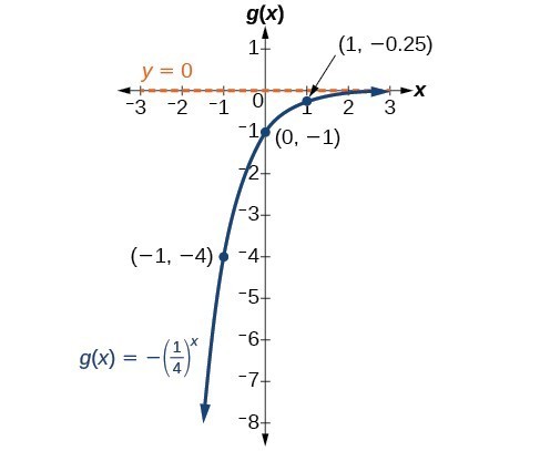
Find and graph the equation for a function, [latex]g\left(x\right)[/latex], that reflects [latex]f\left(x\right)={\left(\frac{1}{4}\right)}^{x}[/latex] about the [latex]x[/latex]-axis. State its domain, range, and asymptote.
Since we want to reflect the parent function [latex]f\left(x\right)={\left(\frac{1}{4}\right)}^{x}[/latex] about the [latex]x[/latex]–axis, we multiply [latex]f\left(x\right)[/latex] by [latex]–1[/latex] to get [latex]g\left(x\right)=-{\left(\frac{1}{4}\right)}^{x}[/latex]. Next we create a table of points.
Plot the [latex]y[/latex]–intercept, [latex]\left(0,-1\right)[/latex], along with two other points. We can use [latex]\left(-1,-4\right)[/latex] and [latex]\left(1,-0.25\right)[/latex].
Draw a smooth curve connecting the points:
The domain is [latex]\left(-\infty ,\infty \right)[/latex], the range is [latex]\left(-\infty ,0\right)[/latex], and the horizontal asymptote is [latex]y=0[/latex].
Summarizing Transformations of the Exponential Function
Now that we have worked with each type of translation for the exponential function, we can summarize them to arrive at the general equation for transforming exponential functions.
Transformations of the Parent Function [latex]f\left(x\right)={b}^{x}[/latex]
A transformation of an exponential function has the form
[latex]f\left(x\right)=a{b}^{x+c}+d[/latex], where the parent function, [latex]y={b}^{x}[/latex], [latex]b>1[/latex], is
shifted horizontally [latex]c[/latex] units to the left.
stretched vertically by a factor of [latex]|a|[/latex] if [latex]|a| > 0[/latex].
compressed vertically by a factor of [latex]|a|[/latex] if [latex]0 < |a| < 1[/latex].
shifted vertically [latex]d[/latex] units.
reflected about the [latex]x[/latex]–axis when [latex]a < 0[/latex].
Note the order of the shifts, transformations, and reflections follow the order of operations.
Write the equation for the function described below. Give the horizontal asymptote, domain, and range.
[latex]f\left(x\right)={e}^{x}[/latex] is vertically stretched by a factor of [latex]2[/latex], reflected across the [latex]y[/latex]-axis, and then shifted up [latex]4[/latex] units.
We want to find an equation of the general form [latex]f\left(x\right)=a{b}^{x+c}+d[/latex]. We use the description provided to find [latex]a, b, c[/latex], and [latex]d[/latex].
We are given the parent function [latex]f\left(x\right)={e}^{x}[/latex], so [latex]b = e[/latex].
The function is stretched by a factor of [latex]2[/latex], so [latex]a = 2[/latex].
The function is reflected about the [latex]y[/latex]-axis. We replace [latex]x[/latex] with [latex]–x[/latex] to get: [latex]{e}^{-x}[/latex].
The graph is shifted vertically [latex]4[/latex] units, so [latex]d = 4[/latex].
The domain is [latex]\left(-\infty ,\infty \right)[/latex]; the range is [latex]\left(4,\infty \right)[/latex]; the horizontal asymptote is [latex]y=4[/latex].