Writing Rational Functions
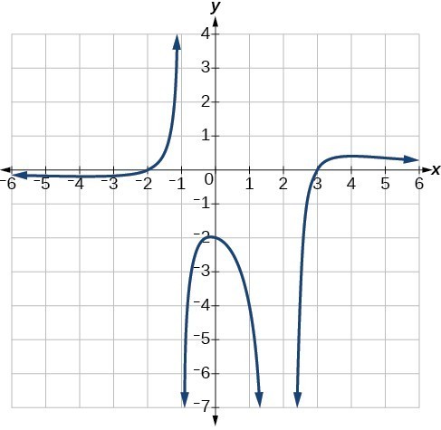
Now that we have analyzed the equations for rational functions and how they relate to a graph of the function, we can use information given by a graph to write the function.
A rational function written in factored form will have an [latex]x[/latex]-intercept where each factor of the numerator is equal to zero. (An exception occurs in the case of a removable discontinuity.) As a result, we can form a numerator of a function whose graph will pass through a set of [latex]x[/latex]-intercepts by introducing a corresponding set of factors. Likewise, because the function will have a vertical asymptote where each factor of the denominator is equal to zero, we can form a denominator that will produce the vertical asymptotes by introducing a corresponding set of factors.
[latex]f\left(x\right)=a\frac{{\left(x-{x}_{1}\right)}^{{p}_{1}}{\left(x-{x}_{2}\right)}^{{p}_{2}}\cdots {\left(x-{x}_{n}\right)}^{{p}_{n}}}{{\left(x-{v}_{1}\right)}^{{q}_{1}}{\left(x-{v}_{2}\right)}^{{q}_{2}}\cdots {\left(x-{v}_{m}\right)}^{{q}_{n}}}[/latex]
where the powers [latex]{p}_{i}[/latex] or [latex]{q}_{i}[/latex] on each factor can be determined by the behavior of the graph at the corresponding intercept or asymptote, and the stretch factor [latex]a[/latex]can be determined given a value of the function other than the [latex]x[/latex]-intercept or by the horizontal asymptote if it is nonzero.
The above example uses an abstract form to help define a rational function. We’ve seen these before.
A linear function can be written in the form [latex]f(x)=mx+b[/latex], and a quadratic function can be written in the form [latex]f(x)=ax^2+bx+c[/latex].
A quadratic can also be written in the form of a polynomial as [latex]p(x)=a(x-r_{1})(x-r_{2})[/latex], where [latex]a[/latex] represents the leading coefficient and [latex]r_{1}[/latex] and [latex]r_{2}[/latex] are the roots, or zeros of the function. Instead of writing “[latex]r_{1}[/latex] and [latex]r_{2}[/latex],” we could use some notational shorthand and simply write, “the [latex]r_{n}[/latex]” to indicate them both at once. That’s the same as saying that the number of roots present include [latex]r_{1}, r_{2}, \ldots, r_{n}[/latex] for [latex]n[/latex] total roots.
In the definition above, to say that “no [latex]x_{i}=\text{ any } v_{j}[/latex]” is to say that there are no common factors in the numerator and denominator. In other words, the roots in the numerator and the vertical asymptotes in the denominator can only be counted in factored and reduced form.
- Determine the factors of the numerator. Examine the behavior of the graph at the x-intercepts to determine the zeroes and their multiplicities. (This is easy to do when finding the “simplest” function with small multiplicities—such as 1 or 3—but may be difficult for larger multiplicities—such as 5 or 7, for example.)
- Determine the factors of the denominator. Examine the behavior on both sides of each vertical asymptote to determine the factors and their powers.
- Use any clear point on the graph to find the stretch factor.

Note in the example above that we used a point on the graph to help write the equation of the graph. In doing so, we used the important concept that any point contained on the graph of a function satisfies the equation of the function (that is, substituting both input and output values into the function equation will result in a true statement).
This concept applies to any function we study. If the function can be graphed in the real plane, it has a set of input [latex]x[/latex] values and a set of corresponding output [latex]f(x)[/latex] values, and each corresponding pair is given by [latex]\left(x, f(x)\right)[/latex].
This correspondence allows us to substitute any [latex]x[/latex] to find its corresponding [latex]f(x)[/latex] and vice versa. It also allows us to substitute both input and output into any function equation in order to solve for a missing third value, such as the leading coefficient [latex]a[/latex] in the example above.
