Using the Intermediate Value Theorem
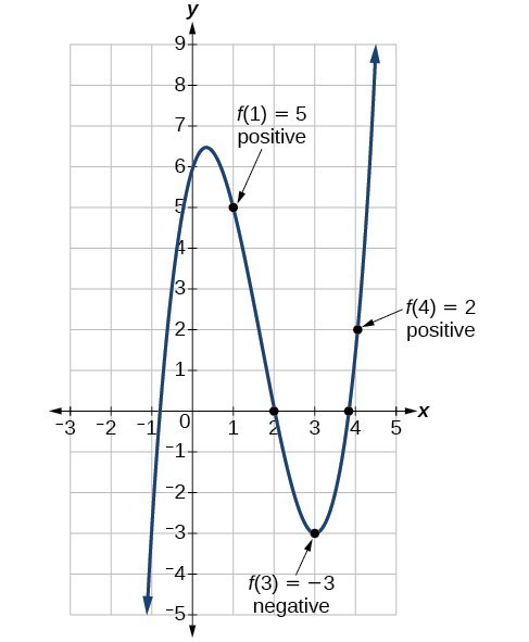
In some situations, we may know two points on a graph but not the zeros. If those two points are on opposite sides of the [latex]x[/latex]-axis, we can confirm that there is a zero between them. Consider a polynomial function [latex]f[/latex] whose graph is smooth and continuous.
Intermediate Value Theorem
The Intermediate Value Theorem states that for two numbers [latex]a[/latex] and [latex]b[/latex] in the domain of [latex]f[/latex], if [latex]a < b[/latex] and [latex]f\left(a\right)\ne f\left(b\right)[/latex], then the function [latex]f[/latex] takes on every value between [latex]f\left(a\right)[/latex] and [latex]f\left(b\right)[/latex].
We can apply this theorem to a special case that is useful for graphing polynomial functions. If a point on the graph of a continuous function f at [latex]x=a[/latex] lies above the [latex]x[/latex]-axis and another point at [latex]x=b[/latex] lies below the [latex]x[/latex]-axis, there must exist a third point between [latex]x=a[/latex] and [latex]x=b[/latex] where the graph crosses the [latex]x[/latex]-axis. Call this point [latex]\left(c,\text{ }f\left(c\right)\right)[/latex]. This means that we are assured there is a value [latex]c[/latex] where [latex]f\left(c\right)=0[/latex].
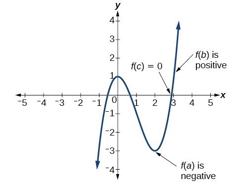
In other words, the Intermediate Value Theorem tells us that when a polynomial function changes from a negative value to a positive value, the function must cross the [latex]x[/latex]-axis. The figure below shows that there is a zero between [latex]a[/latex] and [latex]b[/latex].