- Solve real-world problems involving exponential and logarithmic equations.
- Create models for exponential growth and decay, including how to use Newton’s Law of Cooling and logistic growth.
- Evaluate data to determine the most suitable model, with an emphasis on exponential contexts.
Building a Logarithmic Model from Data
Just as with exponential functions, there are many real-world applications for logarithmic functions: intensity of sound, pH levels of solutions, yields of chemical reactions, production of goods, and growth of infants. As with exponential models, data modeled by logarithmic functions are either always increasing or always decreasing as time moves forward. Again, it is the way they increase or decrease that helps us determine whether a logarithmic model is best.
logarithmic regression
Logarithmic regression is used to model situations where growth or decay accelerates rapidly at first and then slows over time.
The logarithmic equation has the form
[latex]y = a+b \ln(x)[/latex]
where
- all input values, [latex]x[/latex], must be non-negative.
- when [latex]b \gt 0[/latex], the model is increasing.
- when [latex]b \lt 0[/latex], the model is decreasing.
- Use the STAT then EDIT menu to enter given data.
- Clear any existing data from the lists.
- List the input values in the L1 column.
- List the output values in the L2 column.
- Graph and observe a scatter plot of the data using the STATPLOT feature.
- Use ZOOM [9] to adjust axes to fit the data.
- Verify the data follow a logarithmic pattern.
- Find the equation that models the data.
- Select “LnReg” from the STAT then CALC menu.
- Use the values returned for [latex]a[/latex] and [latex]b[/latex] to record the model.
- Graph the model in the same window as the scatterplot to verify it is a good fit for the data.
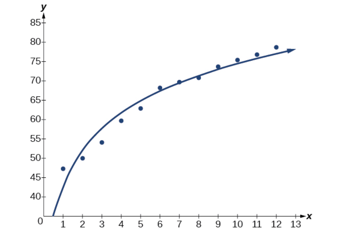
| Year | 1900 | 1910 | 1920 | 1930 | 1940 | 1950 |
| Life Expectancy(Years) | [latex]47.3[/latex] | [latex]50[/latex] | [latex]54.1[/latex] | [latex]59.7[/latex] | [latex]62.9[/latex] | [latex]68.2[/latex] |
| Year | 1960 | 1970 | 1980 | 1990 | 2000 | 2010 |
| Life Expectancy(Years | [latex]69.7[/latex] | [latex]70.8[/latex] | [latex]73.7[/latex] | [latex]75.4[/latex] | [latex]76.8[/latex] | [latex]78.7[/latex] |
- Let [latex]x[/latex] represent time in decades starting with [latex]x = 1[/latex] for the year [latex]1900[/latex], [latex]x= 2[/latex] for the year [latex]1910[/latex], etc. Let [latex]y[/latex] represent the corresponding life expectancy. Use logarithmic regression to fit a model for this data.
- Use the model to predict the average American life expectancy for the year [latex]2030[/latex].
As an environmental scientist, you’re studying noise pollution in urban areas. Sound intensity is measured using decibels (dB), which follow a logarithmic scale. You’re analyzing data to help city planners make informed decisions about noise reduction measures.
A city wants to compare two different methods of analyzing traffic noise. They collected the following data measuring average decibel levels during rush hour:
| Time (hours past 6 AM) | Decibel Level |
|---|---|
| [latex]1[/latex] | [latex]72[/latex] |
| [latex]2[/latex] | [latex]78[/latex] |
| [latex]3[/latex] | [latex]82[/latex] |
| [latex]4[/latex] | [latex]84[/latex] |
| [latex]5[/latex] | [latex]85[/latex] |
Two models have been proposed:
- Model A: [latex]y = 70 + 6.2ln(x)[/latex]
- Model B: [latex]y = 73 + 5.1ln(x)[/latex]
- Calculating the predicted values at hours [latex]1[/latex] and [latex]5[/latex] using both models
- Finding which model has the smaller total error