Graphing a Logarithmic Function Using a Table of Values
Now that we have a feel for the set of values for which a logarithmic function is defined, we move on to graphing logarithmic functions. The family of logarithmic functions includes the parent function [latex]y={\mathrm{log}}_{b}\left(x\right)[/latex] along with all of its transformations: shifts, stretches, compressions, and reflections.
| [latex]x[/latex] | [latex]–3[/latex] | [latex]–2[/latex] | [latex]–1[/latex] | [latex]0[/latex] | [latex]1[/latex] | [latex]2[/latex] | [latex]3[/latex] |
| [latex]{2}^{x}=y[/latex] | [latex]\frac{1}{8}[/latex] | [latex]\frac{1}{4}[/latex] | [latex]\frac{1}{2}[/latex] | [latex]1[/latex] | [latex]2[/latex] | [latex]4[/latex] | [latex]8[/latex] |
| [latex]{\mathrm{log}}_{2}\left(y\right)=x[/latex] | [latex]–3[/latex] | [latex]–2[/latex] | [latex]–1[/latex] | [latex]0[/latex] | [latex]1[/latex] | [latex]2[/latex] | [latex]3[/latex] |
Using the inputs and outputs from the table above, we can build another table to observe the relationship between points on the graphs of the inverse functions [latex]f\left(x\right)={2}^{x}[/latex] and [latex]g\left(x\right)={\mathrm{log}}_{2}\left(x\right)[/latex].
| [latex]f\left(x\right)={2}^{x}[/latex] | [latex]\left(-3,\frac{1}{8}\right)[/latex] | [latex]\left(-2,\frac{1}{4}\right)[/latex] | [latex]\left(-1,\frac{1}{2}\right)[/latex] | [latex]\left(0,1\right)[/latex] | [latex]\left(1,2\right)[/latex] | [latex]\left(2,4\right)[/latex] | [latex]\left(3,8\right)[/latex] |
| [latex]g\left(x\right)={\mathrm{log}}_{2}\left(x\right)[/latex] | [latex]\left(\frac{1}{8},-3\right)[/latex] | [latex]\left(\frac{1}{4},-2\right)[/latex] | [latex]\left(\frac{1}{2},-1\right)[/latex] | [latex]\left(1,0\right)[/latex] | [latex]\left(2,1\right)[/latex] | [latex]\left(4,2\right)[/latex] | [latex]\left(8,3\right)[/latex] |
As we would expect, the [latex]x[/latex]and [latex]y[/latex]-coordinates are reversed for the inverse functions. The figure below shows the graphs of [latex]f[/latex] and [latex]g[/latex].
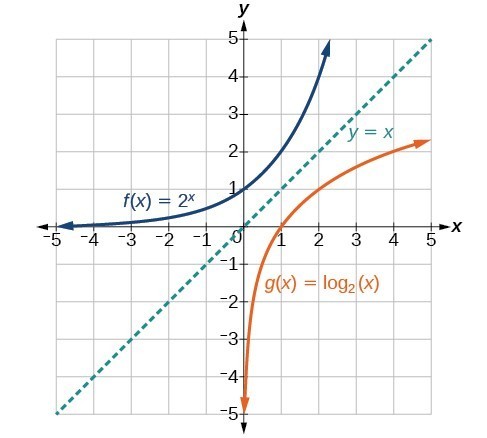
Observe the following from the graph:
- [latex]f\left(x\right)={2}^{x}[/latex] has a y-intercept at [latex]\left(0,1\right)[/latex] and [latex]g\left(x\right)={\mathrm{log}}_{2}\left(x\right)[/latex] has an x-intercept at [latex]\left(1,0\right)[/latex].
- The domain of [latex]f\left(x\right)={2}^{x}[/latex], [latex]\left(-\infty ,\infty \right)[/latex], is the same as the range of [latex]g\left(x\right)={\mathrm{log}}_{2}\left(x\right)[/latex].
- The range of [latex]f\left(x\right)={2}^{x}[/latex], [latex]\left(0,\infty \right)[/latex], is the same as the domain of [latex]g\left(x\right)={\mathrm{log}}_{2}\left(x\right)[/latex].
characteristics of the graph of the parent function [latex]f\left(x\right)={\mathrm{log}}_{b}\left(x\right)[/latex]
For any real number [latex]x[/latex] and constant [latex]b \gt 0[/latex], [latex]b\ne 1[/latex], we can see the following characteristics in the graph of [latex]f\left(x\right)={\mathrm{log}}_{b}\left(x\right)[/latex]:
- one-to-one function
- vertical asymptote: [latex]x = 0[/latex]
- domain: [latex]\left(0,\infty \right)[/latex]
- range: [latex]\left(-\infty ,\infty \right)[/latex]
- [latex]x[/latex]–intercept: [latex]\left(1,0\right)[/latex] and key point [latex]\left(b,1\right)[/latex]
- [latex]y[/latex]-intercept: none
- increasing if [latex]b \gt 1[/latex]
- decreasing if [latex]0 \lt b \lt 1[/latex]
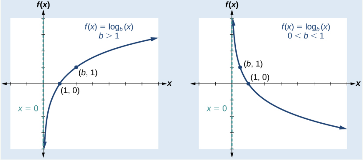
- Draw and label the vertical asymptote, [latex]x = 0[/latex].
- Plot the [latex]x[/latex]–intercept, [latex]\left(1,0\right)[/latex].
- Plot the key point [latex]\left(b,1\right)[/latex].
- Draw a smooth curve through the points.
- State the domain, [latex]\left(0,\infty \right)[/latex], the range, [latex]\left(-\infty ,\infty \right)[/latex], and the vertical asymptote, [latex]x = 0[/latex].

