The Main Idea

• Exponential Growth and Decay:
  • Exponential growth: Increase based on a constant multiplicative rate over equal time increments
  • Exponential decay: Decrease based on a constant multiplicative rate over equal time increments
• Contrast with Linear Growth:
  • Exponential: Changes by the same percentage over equal increments
  • Linear: Changes by the same amount over equal increments
• General Form of Exponential Function:
  • [latex]f(x) = ab^x[/latex]
  • [latex]a[/latex] is any nonzero number
  • [latex]b[/latex] is a positive real number, [latex]b \neq 1[/latex]
  • If [latex]b > 1[/latex]: function grows
  • If [latex]0 < b < 1[/latex]: function decays
• Evaluating Exponential Functions:
  • Substitute the given value for [latex]x[/latex]
  • Follow the order of operations carefully

The Main Idea

• Exponential Growth:
  • Output increases by a constant factor over equal intervals
  • General form: [latex]f(x) = ab^x[/latex], where [latex]b > 1[/latex]
  • Example: [latex]f(x) = 2^x[/latex]
• Exponential Decay:
  • Output decreases by a constant factor over equal intervals
  • General form: [latex]f(x) = ab^x[/latex], where [latex]0 < b < 1[/latex]
  • Example: [latex]g(x) = (\frac{1}{2})^x[/latex]
• Key Characteristics of Exponential Functions:
  • Domain: [latex](-\infty, \infty)[/latex]
  • Range: [latex](0, \infty)[/latex]
  • Horizontal asymptote: [latex]y = 0[/latex]
  • [latex]y[/latex]-intercept: [latex](0, 1)[/latex] for [latex]f(x) = b^x[/latex]
  • No [latex]x[/latex]-intercept

The Main Idea

• General Form of Exponential Functions:
  • [latex]f(x) = ab^x[/latex]
  • [latex]a[/latex]: initial value
  • [latex]b[/latex]: growth factor (if [latex]b > 1[/latex]) or decay factor (if [latex]0 < b < 1[/latex])
• Methods for Finding Equations:
  • Using two points
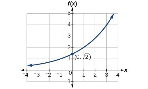
  • Using a graph
• Key Principle:
  • Every point on the graph satisfies the equation of the function

Problem-Solving Strategies

1. When Given Two Points:
   • If one point is [latex](0, a)[/latex], use it as the initial value
   • If no [latex](0, a)[/latex] point, set up a system of equations
2. When Given a Graph:
   • Choose the [latex]y[/latex]-intercept as one point if possible
   • Select a second point with integer coordinates
   • Use points far apart to minimize rounding errors
3. General Steps:
   1. Identify or calculate the initial value [latex]a[/latex]
   2. Use the second point to solve for [latex]b[/latex]
   3. Write the equation in the form [latex]f(x) = ab^x[/latex]

The Main Idea

• Parent Function: [latex]f(x) = b^x[/latex], where [latex]b > 0[/latex] and [latex]b \neq 1[/latex]
• Key Characteristics:
  • Domain: All real numbers [latex](-\infty, \infty)[/latex]
  • Range: All positive real numbers [latex](0, \infty)[/latex]
  • Horizontal asymptote: [latex]y = 0[/latex]
  • y-intercept: [latex](0, 1)[/latex]
  • No x-intercept
• Growth vs. Decay:
  • If [latex]b > 1[/latex]: Exponential growth (increasing function)
  • If [latex]0 < b < 1[/latex]: Exponential decay (decreasing function)

Graphing Strategy

1. Create a table of points:
   • Include negative and positive [latex]x[/latex]-values
   • Always include the [latex]y[/latex]-intercept [latex](0, 1)[/latex]
2. Plot at least [latex]3[/latex] points, including the y-intercept
3. Draw a smooth curve through the points
4. Indicate the horizontal asymptote at [latex]y = 0[/latex]

The Main Idea

• Parent Function: [latex]f(x) = b^x[/latex], where [latex]b > 0[/latex] and [latex]b \neq 1[/latex]
• General Transformed Function: [latex]f(x) = ab^{x-h} + k[/latex]
  • [latex]a[/latex]: Vertical stretch/compression
  • [latex]h[/latex]: Horizontal shift
  • [latex]k[/latex]: Vertical shift
• Key Transformations:
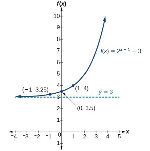
  • Vertical Shift: [latex]f(x) = b^x + d[/latex]
  • Horizontal Shift: [latex]f(x) = b^{x-c}[/latex]

Transformation Effects

1. Vertical Shift ([latex]+d[/latex]):
   • Moves graph up [latex]d[/latex] units if [latex]d > 0[/latex], down if [latex]d < 0[/latex]
   • Changes [latex]y[/latex]-intercept to [latex](0, 1+d)[/latex]
   • Shifts asymptote to [latex]y = d[/latex]
   • New range: [latex](d, \infty)[/latex]
2. Horizontal Shift ([latex]-c[/latex]):
   • Moves graph right [latex]c[/latex] units if [latex]c > 0[/latex], left if [latex]c < 0[/latex]
   • Changes [latex]y[/latex]-intercept to [latex](0, b^c)[/latex]
   • Asymptote remains at [latex]y = 0[/latex]
   • Domain and range unchanged
3. Combined Transformations:
   • Apply horizontal shift first, then vertical shift
   • New [latex]y[/latex]-intercept: [latex](0, b^c + d)[/latex]
   • New asymptote: [latex]y = d[/latex]
   • New range: [latex](d, \infty)[/latex]

Graphing Strategy

1. Identify [latex]b[/latex], [latex]c[/latex], and [latex]d[/latex] in [latex]f(x) = b^{x-c} + d[/latex]
2. Draw the horizontal asymptote [latex]y = d[/latex]
3. Plot the [latex]y[/latex]-intercept [latex](0, b^c + d)[/latex]
4. Sketch the graph, shifting horizontally by [latex]c[/latex] and vertically by [latex]d[/latex]
5. State the domain [latex](-\infty, \infty)[/latex], range [latex](d, \infty)[/latex], and asymptote [latex]y = d[/latex]

The Main Idea

• General Transformed Function: [latex]f(x) = ab^{x-h} + k[/latex]
  • [latex]a[/latex]: Vertical stretch/compression and reflection
  • [latex]b[/latex]: Base of exponential ([latex]b > 0, b \neq 1[/latex])
  • [latex]h[/latex]: Horizontal shift
  • [latex]k[/latex]: Vertical shift
• Vertical Stretch/Compression:
  • [latex]f(x) = ab^x[/latex], where [latex]a \neq 0[/latex]
  • Stretch if [latex]|a| > 1[/latex]
  • Compress if [latex]0 < |a| < 1[/latex]
• Reflections:
  • About [latex]x[/latex]-axis: [latex]f(x) = -b^x[/latex]
  • About [latex]y[/latex]-axis: [latex]f(x) = b^{-x}[/latex]

Transformation Effects

1. Vertical Stretch/Compression ([latex]a[/latex]):
   • Multiplies all [latex]y[/latex]-values by [latex]|a|[/latex]
   • New [latex]y[/latex]-intercept: [latex](0, a)[/latex]
   • Domain and horizontal asymptote unchanged
2. Reflection about [latex]x[/latex]-axis ([latex]-b^x[/latex]):
   • Flips graph upside down
   • New range: [latex](-\infty, 0)[/latex] if [latex]b > 1[/latex], [latex](0, -\infty)[/latex] if [latex]0 < b < 1[/latex]
   • New [latex]y[/latex]-intercept: [latex](0, -1)[/latex]
3. Reflection about [latex]y[/latex]-axis ([latex]b^{-x}[/latex]):
   • Reverses left-right orientation
   • Domain, range, and [latex]y[/latex]-intercept unchanged
   • Growth becomes decay (and vice versa)

Graphing Strategy

1. Identify [latex]a[/latex], [latex]b[/latex], [latex]h[/latex], and [latex]k[/latex] in [latex]f(x) = ab^{x-h} + k[/latex]
2. Apply transformations in this order:
   1. Horizontal shift
   2. Reflection about [latex]y[/latex]-axis (if applicable)
   3. Vertical stretch/compression
   4. Reflection about [latex]x[/latex]-axis (if applicable)
   5. Vertical shift
3. Plot key points: [latex]y[/latex]-intercept and a few others
4. Sketch the curve and asymptote
5. State domain, range, and asymptote