Now that we’ve explored how to find equations of exponential functions, let’s visualize these equations on a graph. Graphing exponential functions allows us to see their behavior clearly, which is crucial for understanding real-world applications like compound interest or population growth.
characteristics of the graph of the parent function [latex]f\left(x\right)={b}^{x}[/latex]
An exponential function with the form [latex]f\left(x\right)={b}^{x}[/latex], [latex]b>0[/latex], [latex]b\ne 1[/latex], has these characteristics:
one-to-one function
The horizontal asymptote is [latex]y = 0[/latex].
The domain of [latex]f[/latex] is all real numbers, [latex](-\infty, \infty)[/latex].
The range of [latex]f[/latex] is all positive real numbers, [latex](0, \infty)[/latex].
There is no [latex]x[/latex]-intercept.
The [latex]y[/latex]-intercept is [latex]\left(0,1\right)[/latex].
The graph is increasing if [latex]b \gt 1[/latex], which implies exponential growth.
The graph decreasing if [latex]0 \lt b \lt 1[/latex], which implies exponential decay.
How To: Given an exponential function of the form [latex]f\left(x\right)={b}^{x}[/latex], graph the function
Create a table of points.
Plot at least [latex]3[/latex] point from the table including the y-intercept [latex]\left(0,1\right)[/latex].
Draw a smooth curve through the points.
State the domain, [latex]\left(-\infty ,\infty \right)[/latex], the range, [latex]\left(0,\infty \right)[/latex], and the horizontal asymptote, [latex]y=0[/latex].
When sketching the graph of an exponential function by plotting points, include a few input values left and right of zero as well as zero itself.
[latex]\\[/latex]
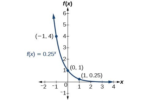
With few exceptions, such as functions that would be undefined at zero or negative input like the radical or (as you’ll see soon) the logarithmic function, it is good practice to let the input equal [latex]-3, -2, -1, 0, 1, 2, \text{ and } 3[/latex] to get the idea of the shape of the graph.Sketch a graph of [latex]f\left(x\right)={0.25}^{x}[/latex]. State the domain, range, and asymptote.
Before graphing, identify the behavior and create a table of points for the graph.
Since [latex]b= 0.25[/latex] is between zero and one, we know the function is decreasing. The left tail of the graph will increase without bound, and the right tail will approach the asymptote [latex]y= 0[/latex].
Create a table of points.
[latex]x[/latex]
[latex]–3[/latex]
[latex]–2[/latex]
[latex]–1[/latex]
[latex]0[/latex]
[latex]1[/latex]
[latex]2[/latex]
[latex]3[/latex]
[latex]f\left(x\right)={0.25}^{x}[/latex]
[latex]64[/latex]
[latex]16[/latex]
[latex]4[/latex]
[latex]1[/latex]
[latex]0.25[/latex]
[latex]0.0625[/latex]
[latex]0.015625[/latex]
Plot the [latex]y[/latex]-intercept, [latex]\left(0,1\right)[/latex], along with two other points. We can use [latex]\left(-1,4\right)[/latex] and [latex]\left(1,0.25\right)[/latex].
Draw a smooth curve connecting the points.
The domain is [latex]\left(-\infty ,\infty \right)[/latex], the range is [latex]\left(0,\infty \right)[/latex], and the horizontal asymptote is [latex]y=0[/latex].
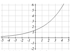
The next example shows how to plot an exponential growth function where the base is greater than [latex]1[/latex].
Sketch a graph of [latex]f(x)={\sqrt{2}(\sqrt{2})}^{x}[/latex]. State the domain and range.
Before graphing, identify the behavior and create a table of points for the graph.
Since [latex]b= \sqrt{2}[/latex], which is greater than one, we know the function is increasing, and we can verify this by creating a table of values. The left tail of the graph will get really close to the x-axis and the right tail will increase without bound.
Plot the [latex]y[/latex]-intercept, [latex]\left(0,1.41\right)[/latex], along with two other points. We can use [latex]\left(-1,1\right)[/latex] and [latex]\left(1,2\right)[/latex].
Draw a smooth curve connecting the points.
Graph of f(x)
The domain is [latex]\left(-\infty ,\infty \right)[/latex]; the range is [latex]\left(0,\infty \right)[/latex].