The Main Idea

• Smoothness: Polynomial functions of degree [latex]2[/latex] or higher have graphs with no sharp corners.
• Continuity: Polynomial graphs have no breaks; they are continuous over their entire domain.
• Domain: All real numbers are valid inputs for polynomial functions.
• Visual Distinction: Polynomial graphs can be distinguished from non-polynomial graphs by their smooth and continuous nature.
• Degree Impact: The degree of the polynomial influences the overall shape and behavior of the graph.

The Main Idea

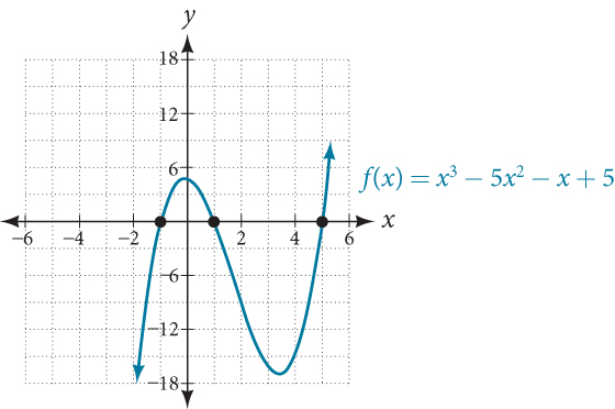
• Zeros Definition: Values of [latex]x[/latex] where [latex]f(x) = 0[/latex] for a polynomial function [latex]f[/latex].
• Zeros correspond to [latex]x[/latex]-intercepts of the polynomial’s graph.
• Factoring Methods:
  • Using known techniques (e.g., greatest common factor, trinomial factoring)
  • Working with pre-factored polynomials
  • Utilizing technology for complex cases
• Set each factor to zero and solve for [latex]x[/latex].
• Each linear factor corresponds to a zero of the polynomial.

The Main Idea

• Zero Definition: Points where a polynomial function crosses or touches the [latex]x[/latex]-axis.
• Multiplicity: The number of times a factor appears in the polynomial’s factored form.
• Behavior at Zeros:
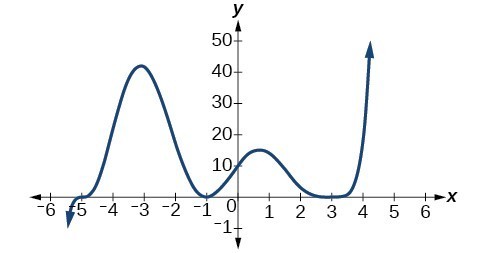
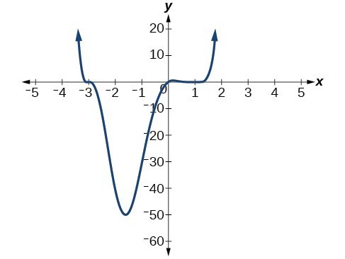
  • Odd multiplicity: Graph crosses the [latex]x[/latex]-axis
  • Even multiplicity: Graph touches or is tangent to the [latex]x[/latex]-axis
• Degree Relationship: The sum of all zero multiplicities equals the polynomial’s degree.
• Graphical Interpretation: The shape of the graph near a zero indicates its multiplicity.

The Main Idea

• Key Elements for Graphing:
  • Zeros and their behavior
  • [latex]y[/latex]-intercepts
  • End behavior
  • Local behavior (turning points and concavity)
• Zeros and Their Multiplicities:
  • Even multiplicity: Graph touches [latex]x[/latex]-axis
  • Odd multiplicity: Graph crosses [latex]x[/latex]-axis
• End Behavior:
  • Determined by the degree (odd or even) and sign of the leading coefficient
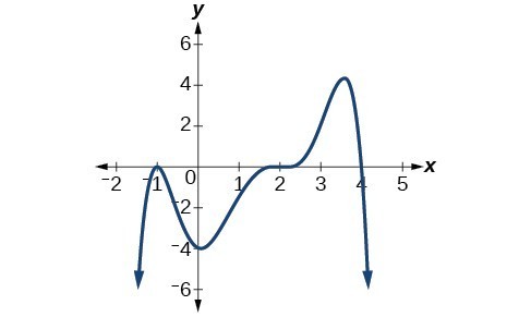
• Turning Points:
  • Maximum number is one less than the polynomial’s degree
• Symmetry:
  • Even functions: Symmetric about [latex]y[/latex]-axis
  • Odd functions: Symmetric about origin

The Main Idea

• Intermediate Value Theorem (IVT): For a continuous function [latex]f(x)[/latex] on [latex][a,b][/latex], if [latex]y[/latex] is between [latex]f(a)[/latex] and [latex]f(b)[/latex], then there exists a [latex]c[/latex] in [latex][a,b][/latex] where [latex]f(c) = y[/latex].
• Application to Zeros: If [latex]f(a)[/latex] and [latex]f(b)[/latex] have opposite signs, there’s at least one zero between [latex]a[/latex] and [latex]b[/latex].
• Helps prove existence of zeros without directly solving equations.
• Continuity: The theorem relies on the function being continuous.

The Main Idea

• Factor Form: [latex]f(x) = a(x-x_1)^{p_1}(x-x_2)^{p_2}...(x-x_n)^{p_n}[/latex]
  • [latex]x_i[/latex] are zeros (x-intercepts)
  • [latex]p_i[/latex] are multiplicities (behavior at zeros)
  • [latex]a[/latex] is the stretch factor
• From Graph to Formula:
  • Identify [latex]x[/latex]-intercepts (zeros)
  • Determine multiplicity at each zero
  • Find stretch factor using another point

Alternative Approaches

1. Reverse Engineering:
   • Start with simple polynomials and modify them to create desired features.
   • Steps:
     • a. Begin with a basic polynomial, e.g., [latex]f(x) = x^3[/latex]
     • b. Add/subtract a constant to shift vertically: [latex]f(x) = x^3 + 2[/latex]
     • c. Add/subtract [latex]x[/latex] to shift horizontally: [latex]f(x) = (x-1)^3 + 2[/latex]
     • d. Multiply by a constant to stretch/compress: [latex]f(x) = 2(x-1)^3 + 2[/latex]
     • e. Add lower-degree terms to adjust shape: [latex]f(x) = 2(x-1)^3 - 3x + 2[/latex]
   • Practice: Start with [latex]f(x) = x^2[/latex] and modify it to match a given graph.
2. Technology-Aided Discovery:
   • Use graphing calculators or software (e.g., Desmos, GeoGebra) to visualize functions.
   • Exploration process:
     • a. Input a general polynomial form: [latex]f(x) = ax^3 + bx^2 + cx + d[/latex]
     • b. Create sliders for coefficients [latex]a[/latex], [latex]b[/latex], [latex]c[/latex], and [latex]d[/latex]
     • c. Adjust sliders to match the given graph
     • d. Observe how each coefficient affects the graph’s shape
   • Advanced: Use parametric equations to visualize how zeros “move” as coefficients change.

The Main Idea

• Local Extrema:
  • Highest/lowest points in an open interval
  • Can be multiple local extrema
• Global Extrema:
  • Highest/lowest points on entire function
  • Only even-degree polynomials have both
• Turning Points:
  • Where function changes from increasing to decreasing or vice versa
  • Maximum number: degree of polynomial minus [latex]1[/latex]