[latex]f\left(x\right)[/latex] is a power function because it can be written as [latex]f\left(x\right)=8{x}^{5}[/latex]. The other functions are not power functions.
Identifying End Behavior of Polynomial Functions
The Main Idea
End behavior describes how a function behaves as [latex]x[/latex] approaches positive or negative infinity.
Even-power functions ([latex]f(x) = ax^n[/latex], [latex]n[/latex] is even):
As [latex]x \to \pm\infty[/latex], [latex]f(x) \to \infty[/latex] if [latex]a > 0[/latex]
As [latex]x \to \pm\infty[/latex], [latex]f(x) \to -\infty[/latex] if [latex]a < 0[/latex]
Odd-power functions ([latex]f(x) = ax^n[/latex], [latex]n[/latex] is odd):
As [latex]x \to -\infty[/latex], [latex]f(x) \to -\infty[/latex] if [latex]a > 0[/latex]
As [latex]x \to \infty[/latex], [latex]f(x) \to \infty[/latex] if [latex]a > 0[/latex]
Behavior is reversed if [latex]a < 0[/latex]
Impact of exponent: Higher powers lead to flatter graphs near the origin and steeper graphs away from it.
Symmetry: Even-power functions are symmetric about the [latex]y[/latex]-axis; odd-power functions are symmetric about the origin.
Describe the end behavior of the graph of [latex]f\left(x\right)=-{x}^{9}[/latex].
The exponent of the power function is 9 (an odd number). Because the coefficient is –1 (negative), the graph is the reflection about the x-axis of the graph of [latex]f\left(x\right)={x}^{9}[/latex]. The graph shows that as x approaches infinity, the output decreases without bound. As x approaches negative infinity, the output increases without bound. In symbolic form, we would write as [latex]x\to -\infty , f\left(x\right)\to \infty[/latex] and as [latex]x\to \infty , f\left(x\right)\to -\infty[/latex].
Graph of f(x)=-x^9
Analysis of the Solution
We can check our work by using the table feature on an online graphing calculator.
Enter the function [latex]f\left(x\right)=-{x}^{9}[/latex] into an online graphing calculator
Create a table with the following x values, and observe the sign of the outputs. [latex]-10,-5,0,5,10[/latex]
Now, enter the function [latex]g\left(x\right)={x}^{9}[/latex], and create a similar table. Compare the signs of the outputs for both functions.
Describe in words and symbols the end behavior of [latex]f\left(x\right)=-5{x}^{4}[/latex].
As [latex]x[/latex] approaches positive or negative infinity, [latex]f\left(x\right)[/latex] decreases without bound: as [latex]x\to \pm \infty , f\left(x\right)\to -\infty[/latex] because of the negative coefficient.
Polynomial Functions
The Main Idea
A polynomial function is of the form [latex]f(x) = a_nx^n + ... + a_2x^2 + a_1x + a_0[/latex], where [latex]n[/latex] is a non-negative integer and [latex]a_i[/latex] are real number coefficients.
Polynomial functions can be created by combining simpler functions, including power functions.
Terms: Each [latex]a_ix^i[/latex] is a term of the polynomial function.
Degree: The highest power of [latex]x[/latex] in the polynomial is its degree.
Degree and Leading Coefficient of a Polynomial Function
The Main Idea
General Form: Polynomials are typically written in descending order of variable powers.
Degree: The highest power of the variable in the polynomial.
Leading Term: The term with the highest degree.
Leading Coefficient: The coefficient of the leading term.
Importance: These concepts help classify and analyze polynomial behavior.
Identify the degree, leading term, and leading coefficient of the polynomial [latex]f\left(x\right)=4{x}^{2}-{x}^{6}+2x - 6[/latex].
The degree is 6. The leading term is [latex]-{x}^{6}[/latex]. The leading coefficient is [latex]–1[/latex].
Watch the following video for more examples of how to determine the degree, leading term, and leading coefficient of a polynomial.
The end behavior of a polynomial is determined by its leading term.
The degree (even or odd) and sign of the leading coefficient determine the specific end behavior pattern.
End behavior is often described using limit notation, such as [latex]\text{as } x \to \infty, f(x) \to \infty[/latex].
To identify end behavior, polynomials should be in expanded (general) form.
The graph of a polynomial function reflects its end behavior.
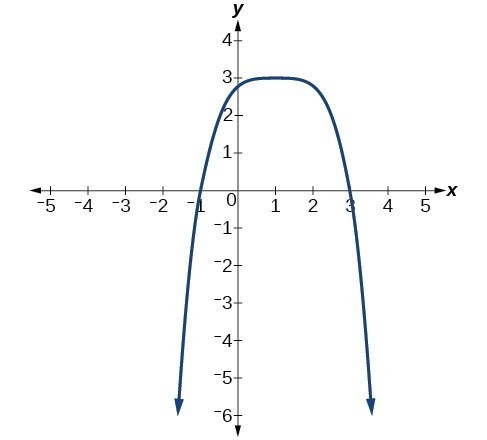
Describe the end behavior of the polynomial function in the graph below.
Graph of a polynomial
As [latex]x\to \infty , f\left(x\right)\to -\infty[/latex] and as [latex]x\to -\infty , f\left(x\right)\to -\infty[/latex]. It has the shape of an even degree power function with a negative coefficient.
In the following video, you’ll see more examples that summarize the end behavior of polynomial functions and which components of the function contribute to it.
Given the function [latex]f\left(x\right)=0.2\left(x - 2\right)\left(x+1\right)\left(x - 5\right)[/latex], express the function as a polynomial in general form and determine the leading term, degree, and end behavior of the function.
The leading term is [latex]0.2{x}^{3}[/latex], so it is a degree 3 polynomial. As x approaches positive infinity, [latex]f\left(x\right)[/latex] increases without bound; as x approaches negative infinity, [latex]f\left(x\right)[/latex] decreases without bound.
Identifying Local Behavior of Polynomial Functions
The Main Idea
Turning Points: Locations where the function changes from increasing to decreasing or vice versa.
Intercepts:
[latex]y[/latex]-intercept: Point where the graph crosses the [latex]y[/latex]-axis [latex](0, a_0)[/latex]
[latex]x[/latex]-intercepts: Points where the graph crosses the [latex]x[/latex]-axis (roots of the polynomial)
Continuity and Smoothness: Polynomial functions are both continuous and smooth.
Degree-Behavior Relationship:
Maximum number of [latex]x[/latex]-intercepts = degree of polynomial
Maximum number of turning points = degree of polynomial – 1
End Behavior: Determined by the degree (odd or even) and the sign of the leading coefficient.
Without graphing the function, determine the maximum number of x-intercepts and turning points for [latex]f\left(x\right)=108 - 13{x}^{9}-8{x}^{4}+14{x}^{12}+2{x}^{3}[/latex]
There are at most 12 x-intercepts and at most 11 turning points.
The following video gives a 5 minute lesson on how to determine the number of intercepts and turning points of a polynomial function given its degree.
The x-intercepts are [latex]\left(0,0\right),\left(-3,0\right)[/latex], and [latex]\left(4,0\right)[/latex].
The degree is 3 so the graph has at most 2 turning points.
Given the function [latex]f\left(x\right)=0.2\left(x - 2\right)\left(x+1\right)\left(x - 5\right)[/latex], determine the local behavior.
The x-intercepts are [latex]\left(2,0\right),\left(-1,0\right)[/latex], and [latex]\left(5,0\right)[/latex], the y-intercept is [latex]\left(0,\text{2}\right)[/latex], and the graph has at most 2 turning points.