Now that we’ve seen and interpreted graphs of linear functions, let’s take a look at how to create the graphs. There are three basic methods of graphing linear functions. The first is by plotting points and then drawing a line through the points. The second is by using the y-intercept and slope. The third is applying transformations to the identity function [latex]f\left(x\right)=x[/latex].
Graphing a Function by Plotting Points
To find points on a function’s graph, select input values, evaluate the function at these inputs, and calculate the corresponding outputs. These input-output pairs form coordinates, which you can plot on a grid. To graph the function, you should evaluate it at least two input values to identify at least two points.
Given the function [latex]f\left(x\right)=2x[/latex], we might use the input values [latex]1[/latex] and [latex]2[/latex].[latex]\\[/latex] Evaluating the function for an input value of [latex]1[/latex] yields an output value of [latex]2[/latex] which is represented by the point [latex](1, 2)[/latex]. [latex]\\[/latex]Evaluating the function for an input value of [latex]2[/latex] yields an output value of [latex]4[/latex] which is represented by the point [latex](2, 4)[/latex].How To: Given a linear function, graph by plotting points.
Choose a minimum of two input values.
Evaluate the function at each input value.
Use the resulting output values to identify coordinate pairs.
Plot the coordinate pairs on a grid.
Draw a line through the points.
Choosing three points is often advisable because if all three points do not fall on the same line, we know we made an error.Graph the following by plotting points.
[latex]f\left(x\right)=-\frac{2}{3}x+5[/latex]
Begin by choosing input values. This function includes a fraction with a denominator of [latex]3[/latex] so let’s choose multiples of [latex]3[/latex] as input values. We will choose [latex]0[/latex], [latex]3[/latex], and [latex]6[/latex].
[latex]\\[/latex]
Evaluate the function at each input value and use the output value to identify coordinate pairs.
Plot the coordinate pairs and draw a line through the points. The graph below is of the function [latex]f\left(x\right)=-\frac{2}{3}x+5[/latex].
Graph of f(x) with three points labeled
Analysis of the Solution
The graph of the function is a line as expected for a linear function. In addition, the graph has a downward slant which indicates a negative slope. This is also expected from the negative constant rate of change in the equation for the function.
Graphing a Linear Function Using [latex]y[/latex]-intercept and Slope
Another way to graph linear functions is by using specific characteristics of the function rather than plotting points. The first characteristic is its [latex]y[/latex]–intercept which is the point at which the input value is zero. To find the [latex]y[/latex]–intercept, we can set [latex]x=0[/latex] in the equation. The other characteristic of the linear function is its slope [latex]m[/latex].
Keep in mind that if a function has a [latex]y[/latex]-intercept, we can always find it by setting [latex]x=0[/latex] and then solving for [latex]y[/latex].Let’s consider the following function.
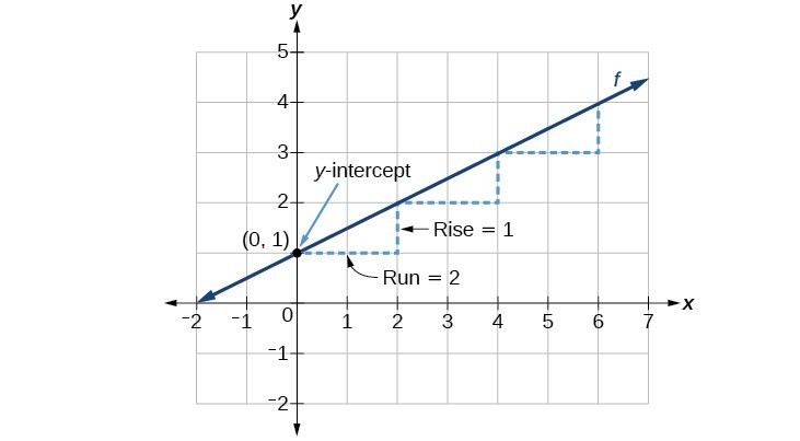
[latex]f\left(x\right)=\frac{1}{2}x+1[/latex]
The slope is [latex]\frac{1}{2}[/latex]. Because the slope is positive, we know the graph will slant upward from left to right.
The [latex]y[/latex]–intercept is the point on the graph when [latex]x = 0[/latex]. The graph crosses the [latex]y[/latex]-axis at [latex](0, 1)[/latex].
Now we know the slope and the [latex]y[/latex]-intercept. We can begin graphing by plotting the point [latex](0, 1)[/latex] We know that the slope is rise over run, [latex]m=\frac{\text{rise}}{\text{run}}[/latex].
From our example, we have [latex]m=\frac{1}{2}[/latex], which means that the rise is [latex]1[/latex] and the run is [latex]2[/latex]. Starting from our [latex]y[/latex]-intercept [latex](0, 1)[/latex], we can rise [latex]1[/latex] and then run [latex]2[/latex] or run [latex]2[/latex] and then rise [latex]1[/latex]. We repeat until we have multiple points, and then we draw a line through the points as shown below.
Graph of f(x) with rise and run labeled
graphical interpretation of a linear function
In the equation [latex]f\left(x\right)=mx+b[/latex]
[latex]b[/latex] is the [latex]y[/latex]-intercept of the graph and indicates the point [latex](0, b)[/latex] at which the graph crosses the [latex]y[/latex]-axis.
[latex]m[/latex] is the slope of the line and indicates the vertical displacement (rise) and horizontal displacement (run) between each successive pair of points. Recall the formula for the slope:
[latex]m=\frac{\text{change in output (rise)}}{\text{change in input (run)}}=\frac{\Delta y}{\Delta x}=\frac{{y}_{2}-{y}_{1}}{{x}_{2}-{x}_{1}}[/latex]
How To: Given the equation for a linear function, graph the function using the [latex]y[/latex]-intercept and slope.
Evaluate the function at an input value of zero to find the [latex]y[/latex]–intercept.
Identify the slope.
Plot the point represented by the y-intercept.
Use [latex]\frac{\text{rise}}{\text{run}}[/latex] to determine at least two more points on the line.
Draw a line which passes through the points.
Graph [latex]f\left(x\right)=-\frac{2}{3}x+5[/latex] using the [latex]y[/latex]–intercept and slope.
Evaluate the function at [latex]x = 0[/latex] to find the [latex]y-[/latex]intercept. The output value when [latex]x = 0[/latex] is [latex]5[/latex], so the graph will cross the [latex]y[/latex]-axis at [latex](0, 5)[/latex].
[latex]\\[/latex]
According to the equation for the function, the slope of the line is [latex]-\frac{2}{3}[/latex]. This tells us that for each vertical decrease in the “rise” of [latex]–2[/latex] units, the “run” increases by [latex]3[/latex] units in the horizontal direction.
[latex]\\[/latex]
We can now graph the function by first plotting the [latex]y[/latex]-intercept. From the initial value [latex](0, 5)[/latex] we move down [latex]2[/latex] units and to the right [latex]3[/latex] units. We can extend the line to the left and right by repeating, and then draw a line through the points.
Graph of f(x)
[latex]\\[/latex] Analysis of the Solution
[latex]\\[/latex]
The graph slants downward from left to right which means it has a negative slope as expected.
![The graph of the linear function [latex]f\left(x\right)=-\frac{2}{3}x+5[/latex].](https://s3-us-west-2.amazonaws.com/courses-images/wp-content/uploads/sites/896/2016/10/21184320/CNX_Precalc_Figure_02_02_0012.jpg)