Representing Linear Functions

Representing a Linear Function in Word Form

Let’s begin by describing the linear function in words. For the train problem we just considered, the following word sentence may be used to describe the function relationship.

• The train’s distance from the station is a function of the time during which the train moves at a constant speed plus its original distance from the station when it began moving at a constant speed.

The speed is the rate of change. Recall that a rate of change is a measure of how quickly the dependent variable changes with respect to the independent variable. The rate of change for this example is constant, which means that it is the same for each input value. As the time (input) increases by [latex]1[/latex] second, the corresponding distance (output) increases by [latex]83[/latex] meters. The train began moving at this constant speed at a distance of [latex]250[/latex] meters from the station.

Representing a Linear Function in Function Notation

Another approach to representing linear functions is by using function notation. One example of function notation is an equation written in the form known as slope-intercept form of a line, where [latex]x[/latex] is the input value, [latex]m[/latex] is the rate of change, and [latex]b[/latex] is the initial value of the dependent variable.

In the example of the train, we might use the notation [latex]D\left(t\right)[/latex] in which the total distance [latex]D[/latex] is a function of the time [latex]t[/latex]. The rate, [latex]m[/latex], is [latex]83[/latex] meters per second. The initial value, [latex]b[/latex], of the dependent variable is the original distance from the station, [latex]250[/latex] meters. We can write a generalized equation to represent the motion of the train.

[latex]D\left(t\right)=83t+250[/latex]

Representing a Linear Function in Tabular Form

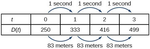
A third method of representing a linear function is through the use of a table. The relationship between the distance from the station and the time is represented in the table below. From the table, we can see that the distance changes by [latex]83[/latex] meters for every [latex]1[/latex] second increase in time.

Representing a Linear Function in Graphical Form

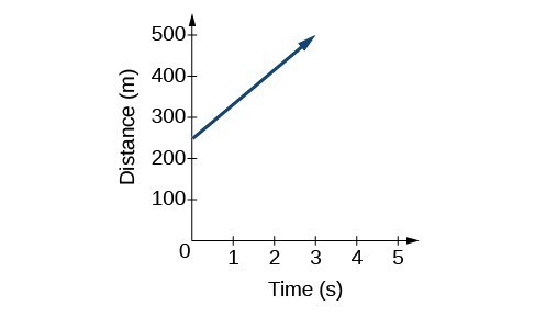
Another way to represent linear functions is visually by using a graph. We can use the function relationship from above, [latex]D\left(t\right)=83t+250[/latex], to draw a graph as seen below. Notice the graph is a line. When we plot a linear function, the graph is always a line.

The rate of change, which is always constant for linear functions, determines the slant or slope of the line. The point at which the input value is zero is the [latex]y[/latex]-intercept of the line. We can see from the graph that the [latex]y[/latex]-intercept in the train example we just saw is [latex]\left(0,250\right)[/latex] and represents the distance of the train from the station when it began moving at a constant speed.

Notice the graph of the train example is restricted since the input value, time, must always be a nonnegative real number. However, this is not always the case for every linear function. Consider the graph of the line [latex]f\left(x\right)=2{x}_{}+1[/latex]. Ask yourself what input values can be plugged into this function, that is, what is the domain of the function? The domain is comprised of all real numbers because any number may be doubled and then have one added to the product.