Shift graphs up, down, left, or right to understand how functions move on the coordinate plane
Flip graphs across the x-axis or y-axis to see how functions mirror themselves
Look at a graph to decide if a function is symmetrical around the y-axis (even), the origin (odd), or not symmetrical at all
Apply compressions and stretches to function graphs
Use different moves and changes like shifting, flipping, squishing, and stretching on graphs
Function transformations are essential tools that help us model and understand real-world situations more accurately. When we learn to shift, stretch, compress, or flip functions, we gain the ability to adapt mathematical models to match real-world scenarios. These transformations are used daily across many fields: engineers design satellite trajectories using shifted parabolas, economists analyze market trends with stretched exponential functions, environmental scientists model climate patterns with transformed trigonometric functions, and medical researchers track disease spread using adjusted logistic curves.
A company monitors the production levels of a factory, where the amount of product produced per hour is represented by the function [latex]P(t)[/latex] with respect to the number of hours ([latex]t[/latex]) since the factory started operations for the day. The production peaks at the midpoint of the shift and then decreases until the end of the shift. Here are three tasks that will transformed the original function this company uses:
Suppose the factory wants to start the operations [latex]2[/latex] hours later than usual.
This corresponds to a horizontal shift to the right by [latex]2[/latex] hours.
New function: [latex]P(t-2)[/latex]
The factory plans to implement new machinery that will halve the time needed to reach peak production.
This corresponds to a horizontal compression by a factor of [latex]2[/latex].
New function: [latex]P(\frac{1}{2}t-2)[/latex]
There is a mandatory maintenance break [latex]4[/latex] hours into the shift, reducing production by [latex]10[/latex] units per hour.
This corresponds to a vertical shift down by [latex]10[/latex] units.
New function: [latex]P(\frac{1}{2}t-2)-10[/latex]
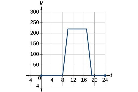
Graph of area of vents open vs. hour in the day
To regulate temperature in a green building, airflow vents near the roof open and close throughout the day. The graph shows the area of open vents [latex]V[/latex] (in square feet) throughout the day in hours after midnight, [latex]t[/latex].
During the summer, the facilities manager decides to try to better regulate temperature by increasing the amount of open vents by [latex]20[/latex] square feet throughout the day and night.Graph this new function.
We can sketch a graph of this new function by adding [latex]20[/latex] to each of the output values of the original function. This will have the effect of shifting the graph vertically up.
Graph of area of vents open vs. hour in the day transposed up 20
Notice that for each input value, the output value has increased by [latex]20[/latex], so if we call the new function [latex]S\left(t\right)[/latex], we could write
[latex]S\left(t\right)=V\left(t\right)+20[/latex]
This notation tells us that, for any value of [latex]t,S\left(t\right)[/latex] can be found by evaluating the function [latex]V[/latex] at the same input and then adding [latex]20[/latex] to the result. This defines [latex]S[/latex] as a transformation of the function [latex]V[/latex], in this case a vertical shift up [latex]20[/latex] units. Notice that, with a vertical shift, the input values stay the same and only the output values change.
[latex]t[/latex]
[latex]0[/latex]
[latex]8[/latex]
[latex]10[/latex]
[latex]17[/latex]
[latex]19[/latex]
[latex]24[/latex]
[latex]V\left(t\right)[/latex]
[latex]0[/latex]
[latex]0[/latex]
[latex]220[/latex]
[latex]220[/latex]
[latex]0[/latex]
[latex]0[/latex]
[latex]S\left(t\right)[/latex]
[latex]20[/latex]
[latex]20[/latex]
[latex]240[/latex]
[latex]240[/latex]
[latex]20[/latex]
[latex]20[/latex]
Suppose that in autumn the facilities manager decides that the original venting plan starts too late, and wants to begin the entire venting program [latex]2[/latex] hours earlier. Graph the new function.
We can set [latex]V\left(t\right)[/latex] to be the original program and [latex]F\left(t\right)[/latex] to be the revised program.
[latex]\begin{align}{c}V\left(t\right)&=\text{ the original venting plan}\\ F\left(t\right)&=\text{starting 2 hrs sooner}\end{align}[/latex]
In the new graph, at each time, the airflow is the same as the original function [latex]V[/latex] was [latex]2[/latex] hours later.
For example, in the original function [latex]V[/latex], the airflow starts to change at [latex]8[/latex] a.m., whereas for the function [latex]F[/latex], the airflow starts to change at [latex]6[/latex] a.m. The comparable function values are [latex]V\left(8\right)=F\left(6\right)[/latex].
Notice also that the vents first opened to [latex]220{\text{ ft}}^{2}[/latex] at [latex]10[/latex] a.m. under the original plan, while under the new plan the vents reach [latex]220{\text{ ft}}^{\text{2}}[/latex] at [latex]8[/latex] a.m., so [latex]V\left(10\right)=F\left(8\right)[/latex].
Graph of area of vents open vs. hour in the day transposed left 2
In both cases, we see that, because [latex]F\left(t\right)[/latex] starts [latex]2[/latex] hours sooner, [latex]h=-2[/latex]. That means that the same output values are reached when [latex]F\left(t\right)=V\left(t-\left(-2\right)\right)=V\left(t+2\right)[/latex].