Rates of Change and Behavior of Graphs: Learn It 1
Find the average rate of change of a function
Identify parts of a graph where the function is going up, going down, or staying the same
Identify the highest and lowest points, both overall and at specific spots, on a graph
Rates of Change
Gasoline costs have experienced some wild fluctuations over the last several decades. The table below[1] lists the average cost, in dollars, of a gallon of gasoline for the years 2014–2023. The cost of gasoline can be considered as a function of year.
[latex]y[/latex]
2014
2015
2016
2017
2018
2019
2020
2021
2022
2023
[latex]C(y)[/latex]
[latex]3.358[/latex]
[latex]2.429[/latex]
[latex]2.143[/latex]
[latex]2.415[/latex]
[latex]2.719[/latex]
[latex]2.604[/latex]
[latex]2.168[/latex]
[latex]3.008[/latex]
[latex]3.951[/latex]
[latex]3.519[/latex]
If we were interested only in how the gasoline prices changed between 2014 and 2023, we could compute that the cost per gallon had increased from [latex]$3.358[/latex] to [latex]$3.519[/latex], an increase of [latex]$0.161[/latex]. While this is interesting, it might be more useful to look at how much the price changed per year. In this section, we will investigate changes such as these.
The price change per year is a rate of change because it describes how an output quantity changes relative to the change in the input quantity. We can see that the price of gasoline in the table above did not change by the same amount each year, so the rate of change was not constant. If we use only the beginning and ending data, we would be finding the average rate of change over the specified period of time. To find the average rate of change, we divide the change in the output value by the change in the input value.
[latex]\begin{align}\text{Average rate of change} &=\frac{\text{Change in output}}{\text{Change in input}}\\[2mm] &=\frac{\Delta y}{\Delta x}\\[2mm] &=\frac{{y}_{2}-{y}_{1}}{{x}_{2}-{x}_{1}}\\[2mm] &=\frac{f\left({x}_{2}\right)-f\left({x}_{1}\right)}{{x}_{2}-{x}_{1}}\end{align}[/latex]
The Greek letter [latex]\Delta[/latex] (delta) signifies the change in a quantity; we read the ratio as “delta-[latex]y[/latex] over delta-[latex]x[/latex]” or “the change in [latex]y[/latex] divided by the change in [latex]x[/latex].” Occasionally we write [latex]\Delta f[/latex] instead of [latex]\Delta y[/latex], which still represents the change in the function’s output value resulting from a change to its input value.
In our example, the gasoline price increased by [latex]$0.161[/latex] from 2014 to 2023. Over [latex]9[/latex] years, the average rate of change was:
On average, the price of gas increased by about [latex]1.79[/latex] cents each year.
Other examples of rates of change include:
A population of rats increasing by [latex]40[/latex] rats per week
A car traveling [latex]68[/latex] miles per hour (distance traveled changes by [latex]68[/latex] miles each hour as time passes)
A car driving [latex]27[/latex] miles per gallon (distance traveled changes by [latex]27[/latex] miles for each gallon)
The current through an electrical circuit increasing by [latex]0.125[/latex] amperes for every volt of increased voltage
The amount of money in a college account decreasing by [latex]$4,000[/latex] per quarter
Rate of Change
A rate of change describes how an output quantity changes relative to the change in the input quantity. The units on a rate of change are “output units per input units.”
[latex]\\[/latex]
The average rate of change between two input values is the total change of the function values (output values) divided by the change in the input values.
How To: Given the value of a function at different points, calculate the average rate of change of a function for the interval between two values [latex]{x}_{1}[/latex] and [latex]{x}_{2}[/latex].
Calculate the difference [latex]{y}_{2}-{y}_{1}=\Delta y[/latex].
Calculate the difference [latex]{x}_{2}-{x}_{1}=\Delta x[/latex].
Find the ratio [latex]\dfrac{\Delta y}{\Delta x}[/latex].
Using the data in the table below, find the average rate of change of the price of gasoline between 2020 and 2022.
[latex]y[/latex]
2014
2015
2016
2017
2018
2019
2020
2021
2022
2023
[latex]C\left(y\right)[/latex]
[latex]3.358[/latex]
[latex]2.429[/latex]
[latex]2.143[/latex]
[latex]2.415[/latex]
[latex]2.719[/latex]
[latex]2.604[/latex]
[latex]2.168[/latex]
[latex]3.008[/latex]
[latex]3.951[/latex]
[latex]3.519[/latex]
In 2020, the price of gasoline was [latex]$2.168[/latex]. In 2022, the cost was [latex]$3.951[/latex]. The average rate of change is:
Note that an increase is expressed by a positive change or “positive increase.” A rate of change is positive when the output increases as the input increases. In this case, we see a significant positive rate of change, indicating a sharp increase in gasoline prices between 2020 and 2022.
After picking up a friend who lives [latex]10[/latex] miles away, Anna records her distance from home over time. The values are shown in the table below. Find her average speed over the first [latex]6[/latex] hours.
t (hours)
[latex]0[/latex]
[latex]1[/latex]
[latex]2[/latex]
[latex]3[/latex]
[latex]4[/latex]
[latex]5[/latex]
[latex]6[/latex]
[latex]7[/latex]
D(t) (miles)
[latex]10[/latex]
[latex]55[/latex]
[latex]90[/latex]
[latex]153[/latex]
[latex]214[/latex]
[latex]240[/latex]
[latex]292[/latex]
[latex]300[/latex]
Here, the average speed is the average rate of change. She traveled [latex]282[/latex] miles in [latex]6[/latex] hours, for an average speed of
The average speed is [latex]47[/latex] miles per hour.
Analysis of the Solution
Because the speed is not constant, the average speed depends on the interval chosen. For the interval [latex][2,3][/latex], the average speed is [latex]63[/latex] miles per hour.
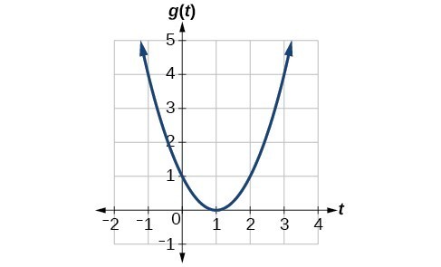
Given the function [latex]g\left(t\right)[/latex], find the average rate of change on the interval [latex]\left[-1,2\right][/latex].
Graph of a parabola
Graph of a parabola with a line and labels
At [latex]t=-1[/latex], the graph shows [latex]g\left(-1\right)=4[/latex]. At [latex]t=2[/latex], the graph shows [latex]g\left(2\right)=1[/latex].The horizontal change [latex]\Delta t=3[/latex] is shown by the red arrow, and the vertical change [latex]\Delta g\left(t\right)=-3[/latex] is shown by the turquoise arrow. The output changes by –3 while the input changes by 3, giving an average rate of change of
Note that the order we choose is very important. If, for example, we use [latex]\dfrac{{y}_{2}-{y}_{1}}{{x}_{1}-{x}_{2}}[/latex], we will not get the correct answer. Decide which point will be 1 and which point will be 2, and keep the coordinates fixed as [latex]\left({x}_{1},{y}_{1}\right)[/latex] and [latex]\left({x}_{2},{y}_{2}\right)[/latex].
Compute the average rate of change of [latex]f\left(x\right)={x}^{2}-\frac{1}{x}[/latex] on the interval [latex]\text{[2,}\text{4].}[/latex]
We can start by computing the function values at each endpoint of the interval.
[latex]\begin{align}\text{Average rate of change}&=\dfrac{f\left(4\right)-f\left(2\right)}{4 - 2} \\[2mm]&=\dfrac{\frac{63}{4}-\frac{7}{2}}{4 - 2} \\[2mm]&=\dfrac{\frac{49}{4}}{2}\\[2mm]&=\dfrac{49}{8}\end{align}[/latex]
The electrostatic force [latex]F[/latex], measured in newtons, between two charged particles can be related to the distance between the particles [latex]d[/latex], in centimeters, by the formula [latex]F\left(d\right)=\frac{2}{{d}^{2}}[/latex]. Find the average rate of change of force if the distance between the particles is increased from [latex]2[/latex] cm to [latex]6[/latex] cm.
We are computing the average rate of change of [latex]F\left(d\right)=\frac{2}{{d}^{2}}[/latex] on the interval [latex]\left[2,6\right][/latex].
The average rate of change is [latex]-\frac{1}{9}[/latex] newton per centimeter.
Find the average rate of change of [latex]g\left(t\right)={t}^{2}+3t+1[/latex] on the interval [latex]\left[0,a\right][/latex]. The answer will be an expression involving [latex]a[/latex].
We use the average rate of change formula.
[latex]\begin{align}\text{Average rate of change}&=\dfrac{g\left(a\right)-g\left(0\right)}{a - 0}&\text{Evaluate}\\[2mm]&=\dfrac{\left({a}^{2}+3a+1\right)-\left({0}^{2}+3\left(0\right)+1\right)}{a - 0}&\text{Simplify}\\[2mm]&=\dfrac{{a}^{2}+3a+1 - 1}{a}&\text{Simplify and factor}\\[2mm]&=\dfrac{a\left(a+3\right)}{a}&\text{Divide by the common factor }a\\[2mm]&=a+3\end{align}[/latex]
This result tells us the average rate of change in terms of [latex]a[/latex] between [latex]t=0[/latex] and any other point [latex]t=a[/latex]. For example, on the interval [latex]\left[0,5\right][/latex], the average rate of change would be [latex]5+3=8[/latex].