Usually a differential equation has infinitely many solutions, so we need to ask: which solution do we actually want? To choose one specific solution, we need more information.
This additional information often comes in the form of an initial value—a condition that tells us the value of the function (and possibly its derivatives) at a specific point.
initial-value problem
An initial-value problem consists of:
A differential equation
One or more initial values (conditions)
Key Rule: The number of initial values needed equals the order of the differential equation.
These problems are called “initial-value problems” because the independent variable often represents time [latex]t[/latex], and [latex]t = 0[/latex] represents the starting point or “initial” moment of the problem.
The initial values allow us to pin down one specific curve from the infinite family of solutions, giving us the particular solution that models our specific situation.
Verify that the function [latex]y=2{e}^{-2t}+{e}^{t}[/latex] is a solution to the initial-value problem
For a function to satisfy an initial-value problem, it must satisfy both the differential equation and the initial condition. To show that [latex]y[/latex] satisfies the differential equation, we start by calculating [latex]{y}^{\prime }[/latex]. This gives [latex]{y}^{\prime }=-4{e}^{-2t}+{e}^{t}[/latex]. Next we substitute both [latex]y[/latex] and [latex]{y}^{\prime }[/latex] into the left-hand side of the differential equation and simplify:
This is equal to the right-hand side of the differential equation, so [latex]y=2{e}^{-2t}+{e}^{t}[/latex] solves the differential equation. Next we calculate [latex]y\left(0\right)\text{:}[/latex]
This result verifies the initial value. Therefore the given function satisfies the initial-value problem.
Watch the following video to see the worked solution to the example above.
For closed captioning, open the video on its original page by clicking the Youtube logo in the lower right-hand corner of the video display. In YouTube, the video will begin at the same starting point as this clip, but will continue playing until the very end.You can view the transcript for this segmented clip of “4.1.5” here (opens in new window).
The initial-value problem in the previous example consisted of two essential parts:
The differential equation: [latex]y' + 2y = 3e^t[/latex]
The initial condition: [latex]y(0) = 3[/latex]
Together, these two pieces formed the complete initial-value problem.
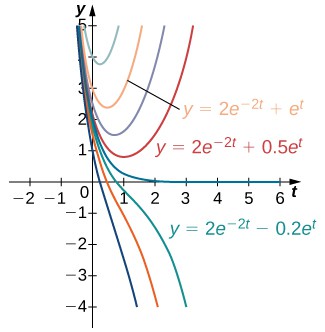
For our example, the general solution to the differential equation [latex]y' + 2y = 3e^t[/latex] is [latex]y = 2e^{-2t} + Ce^t[/latex]. This represents an entire family of curves, each corresponding to a different value of [latex]C[/latex].
The initial condition [latex]y(0) = 3[/latex] tells us which curve from this family we actually want. When we substitute [latex]t = 0[/latex] and [latex]y = 3[/latex] into the general solution, we find that [latex]C = 1[/latex], giving us the particular solution [latex]y = 2e^{-2t} + e^t[/latex].
Figure 2 shows this family of solutions, with our particular solution highlighted. You can see how the initial condition picks out exactly one curve from the infinite family.
Figure 2: A family of solutions to the differential equation y′+2y=3et. The particular solution y=2e−2t+et is labeled.
The first step in solving this initial-value problem is to find a general family of solutions. To do this, we find an antiderivative of both sides of the differential equation
We are able to integrate both sides because the y term appears by itself. Notice that there are two integration constants: [latex]{C}_{1}[/latex] and [latex]{C}_{2}[/latex]. Solving the previous equation for [latex]y[/latex] gives
Because [latex]{C}_{1}[/latex] and [latex]{C}_{2}[/latex] are both constants, [latex]{C}_{2}-{C}_{1}[/latex] is also a constant. We can therefore define [latex]C={C}_{2}-{C}_{1}[/latex], which leads to the equation
Next we determine the value of [latex]C[/latex]. To do this, we substitute [latex]x=0[/latex] and [latex]y=5[/latex] into our aforementioned equation and solve for [latex]C\text{:}[/latex]
Now we substitute the value [latex]C=2[/latex] into our equation. The solution to the initial-value problem is [latex]y=3{e}^{x}+\frac{1}{3}{x}^{3}-4x+2[/latex].
Analysis
The difference between a general solution and a particular solution is that a general solution involves a family of functions, either explicitly or implicitly defined, of the independent variable. The initial value or values determine which particular solution in the family of solutions satisfies the desired conditions.
Watch the following video to see the worked solution to example above.
For closed captioning, open the video on its original page by clicking the Youtube logo in the lower right-hand corner of the video display. In YouTube, the video will begin at the same starting point as this clip, but will continue playing until the very end.You can view the transcript for this segmented clip of “4.1.5” here (opens in new window).