Limit of a Sequence
Now that we understand what sequences are, let’s explore a fundamental question: What happens to the terms of a sequence as [latex]n[/latex] gets larger and larger?
Since sequences are functions defined on positive integers, we can discuss what happens to [latex]a_n[/latex] as [latex]n \to \infty[/latex]. Let’s examine four different sequences to see the various behaviors that can occur.
Example a: [latex]{1+3n} = {4, 7, 10, 13, \ldots}[/latex]
The terms [latex]1+3n[/latex] grow without bound as [latex]n \to \infty[/latex]. We say [latex]1+3n \to \infty[/latex] as [latex]n \to \infty[/latex].
Example b: [latex]{1-(\frac{1}{2})^n} = {\frac{1}{2}, \frac{3}{4}, \frac{7}{8}, \frac{15}{16}, \ldots}[/latex]
The terms get closer and closer to 1. We say [latex]1-(\frac{1}{2})^n \to 1[/latex] as [latex]n \to \infty[/latex].
Example c: [latex]{(-1)^n} = {-1, 1, -1, 1, \ldots}[/latex]
The terms alternate between -1 and 1 forever. They don’t settle down to any single value.
Example d: [latex]{\frac{(-1)^n}{n}} = {-1, \frac{1}{2}, -\frac{1}{3}, \frac{1}{4}, \ldots}[/latex]
The terms alternate in sign but get closer and closer to 0. We say [latex]\frac{(-1)^n}{n} \to 0[/latex] as [latex]n \to \infty[/latex].
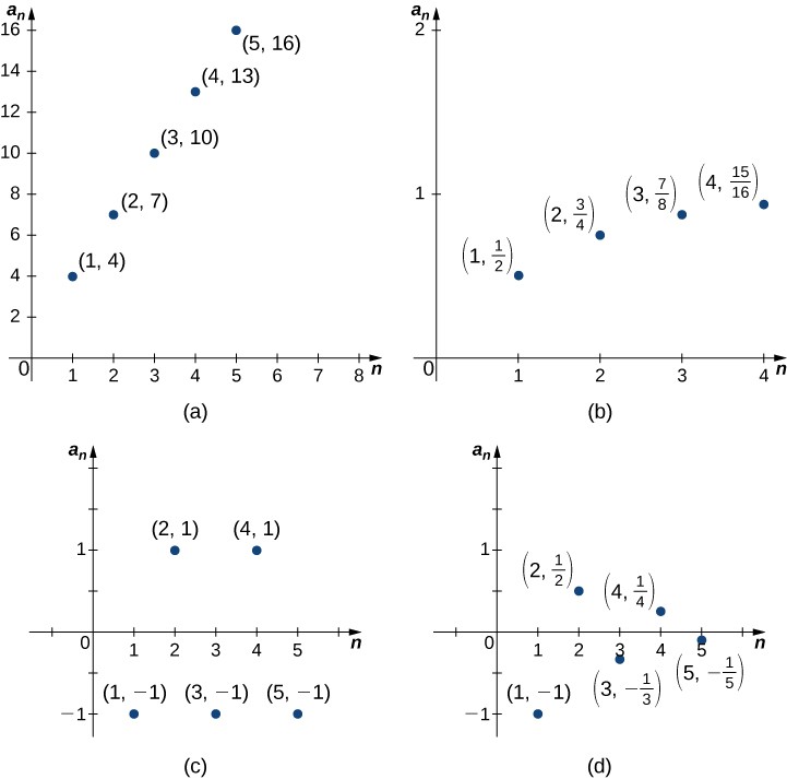
From these examples, we see that sequences can behave in different ways as [latex]n[/latex] gets large. In Examples b and c, the terms approach a specific finite number. In Examples a and c, they don’t. If the terms of a sequence approach a finite number [latex]L[/latex] as [latex]n\to \infty[/latex], we say that the sequence is a convergent sequence and the real number [latex]L[/latex] is the limit of the sequence.
convergent and divergent sequences
A sequence [latex]{a_n}[/latex] is convergent if the terms [latex]a_n[/latex] get arbitrarily close to some finite number [latex]L[/latex] as [latex]n[/latex] becomes sufficiently large.
We write:
[latex]\lim_{n\to \infty}a_n = L[/latex]
The number [latex]L[/latex] is called the limit of the sequence.
If a sequence is not convergent, we say it is divergent.
Convergent vs. Divergent
- Convergent: The terms “settle down” to approach a specific finite value
- Divergent: The terms either grow without bound, oscillate forever, or behave erratically
Remember: Even if terms alternate (like in Example 4), a sequence can still converge if the alternating terms get closer to a single value.
Looking at our examples more closely, we can see that [latex]{1-(\frac{1}{2})^n}[/latex] has terms that get arbitrarily close to 1 as [latex]n[/latex] becomes very large. This makes it a convergent sequence with limit 1. In contrast, [latex]{1+3n}[/latex] has terms that keep growing without approaching any finite number, making it divergent.
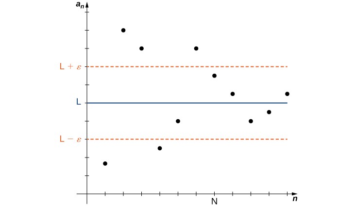
The Formal Definition
Our informal description used phrases like “arbitrarily close” and “sufficiently large,” which are helpful but somewhat vague. Here’s the precise mathematical definition and show these ideas graphically in Figure 3.
formal definition of sequence convergence
A sequence [latex]{a_n}[/latex] converges to a real number [latex]L[/latex] if:
For every [latex]\epsilon > 0[/latex], there exists an integer [latex]N[/latex] such that [latex]|a_n - L| < \epsilon[/latex] whenever [latex]n \geq N[/latex].
We write:
[latex]\underset{n\to \infty }{\text{lim}}a_n = L[/latex] or [latex]a_n \to L[/latex]
If a sequence doesn’t converge, it’s divergent.
The convergence of a sequence depends only on what happens as [latex]n \to \infty[/latex]. This means you can add or remove any finite number of terms from the beginning of a sequence without changing whether it converges or diverges.
Not all divergent sequences behave the same way. Let’s look at the sequences [latex]{1+3n}[/latex] and [latex]{(-1)^n}[/latex] from our earlier examples to see two distinct types of divergence.
Oscillating divergence: The sequence [latex]{(-1)^n} = {-1, 1, -1, 1, \ldots}[/latex] diverges because terms alternate between 1 and -1 forever, never settling on a single value.
Divergence to infinity: The sequence [latex]{1+3n}[/latex] diverges because the terms grow without bound: [latex]1+3n \to \infty[/latex] as [latex]n \to \infty[/latex].
For sequences that grow without bound, we write [latex]\lim_{n\to \infty}(1+3n) = \infty[/latex]. Similarly, sequences can diverge to negative infinity. For example, [latex]{-5n+2}[/latex] has terms that approach [latex]-\infty[/latex], so we write [latex]\lim_{n\to \infty}(-5n+2) = -\infty[/latex].
Important Note About Infinity
When we write [latex]\lim_{n\to \infty}a_n = \infty[/latex], we’re not saying the limit exists. The sequence is still divergent! This notation just tells us how it diverges—by growing without bound rather than oscillating.
Using Function Limits to Find Sequence Limits
Since sequences are functions defined on positive integers, we can often use our knowledge of function limits to analyze sequence behavior.
Here’s the key insight: If you have a sequence [latex]{a_n}[/latex] where [latex]a_n = f(n)[/latex] for some function [latex]f[/latex], and if [latex]\lim_{x\to \infty}f(x) = L[/latex], then the sequence converges to the same limit [latex]L[/latex].
limit of a sequence defined by a function
Consider a sequence [latex]\left\{{a}_{n}\right\}[/latex] such that [latex]{a}_{n}=f\left(n\right)[/latex] for all [latex]n\ge 1[/latex]. If there exists a real number [latex]L[/latex] such that
then [latex]\left\{{a}_{n}\right\}[/latex] converges and
This method is especially useful when:
- Your sequence formula looks like a familiar function
- You can easily find the limit of the continuous version
- The function techniques (like L’Hôpital’s rule) are simpler than working directly with the sequence