First-Order Linear Equations and Applications: Apply It

Giselle Miller

First-Order Linear Equations and Applications: Apply It

Write first-order linear differential equations in their standard form
Find and use integrating factors to solve first-order linear equations
Understand how carrying capacity affects population growth in the logistic model
Work with logistic equations and interpret what their solutions mean
Solve real-world problems using first-order linear differential equations

Applications of First-order Linear Differential Equations

We look at two different applications of first-order linear differential equations. The first involves air resistance as it relates to objects that are rising or falling; the second involves an electrical circuit. Other applications are numerous, but most are solved in a similar fashion.

Free fall with air resistance

We discussed air resistance at the beginning of this section. The next example shows how to apply this concept for a ball in vertical motion. Other factors can affect the force of air resistance, such as the size and shape of the object, but we ignore them here.

A racquetball is hit straight upward with an initial velocity of [latex]2[/latex] m/s. The mass of a racquetball is approximately [latex]0.0427[/latex] kg. Air resistance acts on the ball with a force numerically equal to [latex]0.5v[/latex], where [latex]v[/latex] represents the velocity of the ball at time [latex]t[/latex].

Find the velocity of the ball as a function of time.
How long does it take for the ball to reach its maximum height?
If the ball is hit from an initial height of [latex]1[/latex] meter, how high will it reach?

The mass [latex]m=0.0427\text{kg},k=0.5[/latex], and [latex]g=9.8{\text{m/s}}^{2}[/latex]. The initial velocity is [latex]{v}_{0}=2[/latex] m/s. Therefore the initial-value problem is

[latex]0.0427\frac{dv}{dt}=-0.5v - 0.0427\left(9.8\right),{v}_{0}=2[/latex].

Dividing the differential equation by [latex]0.0427[/latex] gives

[latex]\frac{dv}{dt}=-11.7096v - 9.8,{v}_{0}=2[/latex].

The differential equation is linear. Using the problem-solving strategy for linear differential equations:

Step 1. Rewrite the differential equation as [latex]\frac{dv}{dt}+11.7096v=-9.8[/latex]. This gives [latex]p\left(t\right)=11.7096[/latex] and [latex]q\left(t\right)=-9.8[/latex]

Step 2. The integrating factor is [latex]\mu \left(t\right)={e}^{\displaystyle\int 11.7096dt}={e}^{11.7096t}[/latex].

Step 3. Multiply the differential equation by [latex]\mu \left(t\right)\text{:}[/latex]

[latex]\begin{array}{ccc}\hfill {e}^{11.7096t}\frac{dv}{dt}+11.7096v{e}^{11.7096t}& =\hfill & -9.8{e}^{11.7096t}\hfill \\ \hfill \frac{d}{dt}\left[v{e}^{11.7096t}\right]& =\hfill & -9.8{e}^{11.7096t}.\hfill \end{array}[/latex]

Step 4. Integrate both sides:

[latex]\begin{array}{ccc}\hfill {\displaystyle\int \frac{d}{dt}\left[v{e}^{11.7096t}\right]dt}& =\hfill & {\displaystyle\int -9.8{e}^{11.7096t}dt}\hfill \\ \hfill v{e}^{11.7096t}& =\hfill & \frac{-9.8}{11.7096}{e}^{11.7096t}+C\hfill \\ \hfill v\left(t\right)& =\hfill & -0.8369+C{e}^{-11.7096t}.\hfill \end{array}[/latex]

Step 5. Solve for [latex]C[/latex] using the initial condition [latex]{v}_{0}=v\left(0\right)=2\text{:}[/latex]

[latex]\begin{array}{ccc}\hfill v\left(t\right)& =\hfill & -0.8369+C{e}^{-11.7096t}\hfill \\ \hfill v\left(0\right)& =\hfill & -0.8369+C{e}^{-11.7096\left(0\right)}\hfill \\ \hfill 2& =\hfill & -0.8369+C\hfill \\ \hfill C& =\hfill & 2.8369.\hfill \end{array}[/latex]

Therefore the solution to the initial-value problem is [latex]v\left(t\right)=2.8369{e}^{-11.7096t}-0.8369[/latex].
The ball reaches its maximum height when the velocity is equal to zero. The reason is that when the velocity is positive, it is rising, and when it is negative, it is falling. Therefore when it is zero, it is neither rising nor falling, and is at its maximum height:

[latex]\begin{array}{}\\ \hfill 2.8369{e}^{-11.7096t}-0.8369& =\hfill & 0\hfill \\ \hfill 2.8369{e}^{-11.7096t}& =\hfill & 0.8369\hfill \\ \hfill {e}^{-11.7096t}& =\hfill & \frac{0.8369}{2.8369}\approx 0.295\hfill \\ \hfill \text{ln}{e}^{-11.7096t}& =\hfill & \text{ln}0.295\approx -1.221\hfill \\ \hfill -11.7096t& =\hfill & -1.221\hfill \\ \hfill t& \approx \hfill & 0.104.\hfill \end{array}[/latex]

Therefore it takes approximately [latex]0.104[/latex] second to reach maximum height.
To find the height of the ball as a function of time, use the fact that the derivative of position is velocity, i.e., if [latex]h\left(t\right)[/latex] represents the height at time [latex]t[/latex], then [latex]{h}^{\prime }\left(t\right)=v\left(t\right)[/latex]. Because we know [latex]v\left(t\right)[/latex] and the initial height, we can form an initial-value problem:

[latex]{h}^{\prime }\left(t\right)=2.8369{e}^{-11.7096t}-0.8369,h\left(0\right)=1[/latex].

Integrating both sides of the differential equation with respect to [latex]t[/latex] gives

[latex]\begin{array}{ccc}\hfill {\displaystyle\int {h}^{\prime }\left(t\right)dt}& =\hfill & {\displaystyle\int 2.8369{e}^{-11.7096t}-0.8369dt}\hfill \\ \hfill h\left(t\right)& =\hfill & -\frac{2.8369}{11.7096}{e}^{-11.7096t}-0.8369t+C\hfill \\ \hfill h\left(t\right)& =\hfill & -0.2423{e}^{-11.7096t}-0.8369t+C.\hfill \end{array}[/latex]

Solve for [latex]C[/latex] by using the initial condition:

[latex]\begin{array}{ccc}\hfill h\left(t\right)& =\hfill & -0.2423{e}^{-11.7096t}-0.8369t+C\hfill \\ \hfill h\left(0\right)& =\hfill & -0.2423{e}^{-11.7096\left(0\right)}-0.8369\left(0\right)+C\hfill \\ \hfill 1& =\hfill & -0.2423+C\hfill \\ \hfill C& =\hfill & 1.2423.\hfill \end{array}[/latex]

Therefore

[latex]h\left(t\right)=-0.2423{e}^{-11.7096t}-0.8369t+1.2423[/latex].

After [latex]0.104[/latex] second, the height is given by

[latex]h\left(0.2\right)=-0.2423{e}^{-11.7096t}-0.8369t+1.2423\approx 1.0836[/latex] meter.

Watch the following video to see the worked solution to the example above.

For closed captioning, open the video on its original page by clicking the Youtube logo in the lower right-hand corner of the video display. In YouTube, the video will begin at the same starting point as this clip, but will continue playing until the very end.

You can view the transcript for this segmented clip of “4.5.3” here (opens in new window).

The weight of a penny is [latex]2.5[/latex] grams (United States Mint, “Coin Specifications,” accessed April 9, 2015, http://www.usmint.gov/about_the_mint/?action=coin_specifications), and the upper observation deck of the Empire State Building is [latex]369[/latex] meters above the street. Since the penny is a small and relatively smooth object, air resistance acting on the penny is actually quite small. We assume the air resistance is numerically equal to [latex]0.0025v[/latex]. Furthermore, the penny is dropped with no initial velocity imparted to it.

Set up an initial-value problem that represents the falling penny.
Solve the problem for [latex]v\left(t\right)[/latex].
What is the terminal velocity of the penny (i.e., calculate the limit of the velocity as [latex]t[/latex] approaches infinity)?

Electrical Circuits

Electrical circuits involve the flow of current through various components, each creating specific voltage drops. Understanding these relationships allows engineers to analyze and design everything from simple household circuits to complex electronic devices.

When a source of electromotive force (like a battery or generator) drives current through a closed circuit, that current encounters resistance, inductance, and capacitance. Each of these circuit elements affects the voltage in predictable ways.

Kirchhoff’s Loop Rule states that the sum of all voltage drops around any closed circuit loop equals the total electromotive force. This fundamental principle lets us set up equations that describe circuit behavior.

The voltage drop across each type of circuit element follows specific patterns:

Resistor: [latex]E_R = Ri[/latex]

[latex]R[/latex] = resistance (a constant)
[latex]i[/latex] = current

Inductor: [latex]E_L = Li'[/latex]

[latex]L[/latex] = inductance (a constant)
[latex]i'[/latex] = rate of change of current

Capacitor: [latex]E_C = \frac{1}{C}q[/latex]

[latex]C[/latex] = capacitance (a constant)
[latex]q[/latex] = instantaneous charge

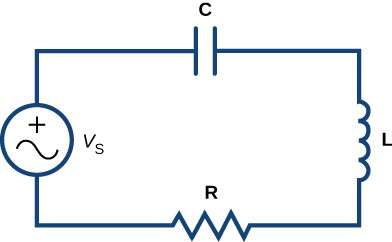
The circuit shown below contains all three types of components: a voltage source ([latex]V_S[/latex]), capacitor ([latex]C[/latex]), inductor ([latex]L[/latex]), and resistor ([latex]R[/latex]). This configuration allows us to analyze how differential equations emerge from physical circuit laws.

A diagram of an electric circuit in a rectangle. The top has a capacitor C, the left has a voltage generator Vs, the bottom was a resistor R, and the right has an inductor L.

Understanding the units helps ensure your calculations make physical sense:

Voltage [latex]E[/latex]: volts (V)
Current [latex]i[/latex]: amperes (A)
Charge [latex]q[/latex]: coulombs (C)
Resistance [latex]R[/latex]: ohms (Ω)
Inductance [latex]L[/latex]: henrys (H)
Capacitance [latex]C[/latex]: farads (F)

Applying Kirchhoff’s Loop Rule to this circuit, we let [latex]E[/latex] denote the electromotive force supplied by the voltage generator. Then

[latex]{E}_{L}+{E}_{R}+{E}_{C}=E[/latex].

Substituting the expressions for [latex]{E}_{L},{E}_{R}[/latex], and [latex]{E}_{C}[/latex] into this equation, we obtain

[latex]L{i}^{\prime }+Ri+\frac{1}{C}q=E[/latex].

If there is no capacitor in the circuit, then the equation becomes

[latex]L{i}^{\prime }+Ri=E[/latex].

This is a first-order differential equation in [latex]i[/latex]. The circuit is referred to as an [latex]LR[/latex] circuit.

Next, suppose there is no inductor in the circuit, but there is a capacitor and a resistor, so [latex]L=0,R\ne 0[/latex], and [latex]C\ne 0[/latex]. Then [latex]y=\dfrac{1}{\mu \left(x\right)}\left[\displaystyle\int \mu \left(x\right)q\left(x\right)dx+C\right][/latex] can be rewritten as

[latex]R{q}^{\prime }+\frac{1}{C}q=E[/latex],

which is a first-order linear differential equation. This is referred to as an [latex]RC[/latex] circuit. In either case, we can set up and solve an initial-value problem.

A circuit has in series an electromotive force given by [latex]E=50\sin{20t}\text{ V}[/latex], a resistor of [latex]5 \Omega[/latex], and an inductor of [latex]0.4\text{H}\text{.}[/latex] If the initial current is [latex]0[/latex], find the current at time [latex]t>0[/latex].

We have a resistor and an inductor in the circuit, so we use [latex]L{i}^{\prime }+Ri+\frac{1}{C}q=E[/latex]. The voltage drop across the resistor is given by [latex]{E}_{R}=Ri=5i[/latex]. The voltage drop across the inductor is given by [latex]{E}_{L}=L{i}^{\prime }=0.4{i}^{\prime }[/latex]. The electromotive force becomes the right-hand side of the equation. Therefore the equation becomes

[latex]0.4{i}^{\prime }+5i=50\sin{20t}[/latex].

Dividing both sides by [latex]0.4[/latex] gives the equation

[latex]{i}^{\prime }+12.5i=125\sin{20t}[/latex].

Since the initial current is 0, this result gives an initial condition of [latex]i\left(0\right)=0[/latex]. We can solve this initial-value problem using the five-step strategy for solving first-order differential equations.

Step 1. Rewrite the differential equation as [latex]{i}^{\prime }+12.5i=125\sin{20t}[/latex]. This gives [latex]p\left(t\right)=12.5[/latex] and [latex]q\left(t\right)=125\sin20t[/latex].

Step 2. The integrating factor is [latex]\mu \left(t\right)={e}^{\displaystyle\int 12.5dt}={e}^{12.5t}[/latex].

Step 3. Multiply the differential equation by [latex]\mu \left(t\right)\text{:}[/latex]

[latex]\begin{array}{ccc}\hfill {e}^{12.5t}{i}^{\prime }+12.5{e}^{12.5t}i& =\hfill & 125{e}^{12.5t}\sin20t\hfill \\ \hfill \frac{d}{dt}\left[i{e}^{12.5t}\right]& =\hfill & 125{e}^{12.5t}\sin20t.\hfill \end{array}[/latex]

Step 4. Integrate both sides:

[latex]\begin{array}{ccc}\hfill {\displaystyle\int \frac{d}{dt}\left[i{e}^{12.5t}\right]dt}& =\hfill & {\displaystyle\int 125{e}^{12.5t}\sin{20t}dt}\hfill \\ \hfill i{e}^{12.5t}& =\hfill & \left(\frac{250\sin{20t} - 400\cos{20t}}{89}\right){e}^{12.5t}+C\hfill \\ \hfill i\left(t\right)& =\hfill & \frac{250\sin20t - 400\cos20t}{89}+C{e}^{-12.5t}.\hfill \end{array}[/latex]

Step 5. Solve for [latex]C[/latex] using the initial condition [latex]v\left(0\right)=2\text{:}[/latex]

[latex]\begin{array}{ccc}\hfill i\left(t\right)& =\hfill & \frac{250\sin{20t} - 400\cos{20t}}{89}+C{e}^{-12.5t}\hfill \\ \hfill i\left(0\right)& =\hfill & \frac{250\sin{20}\left(0\right)-400\cos{20}\left(0\right)}{89}+C{e}^{-12.5\left(0\right)}\hfill \\ \hfill 0& =\hfill & -\frac{400}{89}+C\hfill \\ \hfill C& =\hfill & \frac{400}{89}.\hfill \end{array}[/latex]

Therefore the solution to the initial-value problem is [latex]i\left(t\right)=\frac{250\sin{20t} - 400\cos{20t}+400{e}^{-12.5t}}{89}=\frac{250\sin{20t} - 400\cos{20t}}{89}+\frac{400{e}^{-12.5t}}{89}[/latex].

The first term can be rewritten as a single cosine function. First, multiply and divide by [latex]\sqrt{{250}^{2}+{400}^{2}}=50\sqrt{89}\text{:}[/latex]

[latex]\begin{array}{cc}\hfill \frac{250\sin{20t} - 400\cos{20t}}{89}& =\frac{50\sqrt{89}}{89}\left(\frac{250\sin{20t} - 400\cos{20t}}{50\sqrt{89}}\right)\hfill \\ & =-\frac{50\sqrt{89}}{89}\left(\frac{8\cos{20t}}{\sqrt{89}}-\frac{5\sin{20t}}{\sqrt{89}}\right).\hfill \end{array}[/latex]

Next, define [latex]\phi[/latex] to be an acute angle such that [latex]\cos\phi =\frac{8}{\sqrt{89}}[/latex]. Then [latex]\sin\phi =\frac{5}{\sqrt{89}}[/latex] and

[latex]\begin{array}{cc}\hfill -\frac{50\sqrt{89}}{89}\left(\frac{8\cos20t}{\sqrt{89}}-\frac{5\sin20t}{\sqrt{89}}\right)& =-\frac{50\sqrt{89}}{89}\left(\cos\phi \cos20t-\sin\phi \sin20t\right)\hfill \\ & =-\frac{50\sqrt{89}}{89}\cos\left(20t+\phi \right).\hfill \end{array}[/latex]

Therefore the solution can be written as

[latex]i\left(t\right)=-\frac{50\sqrt{89}}{89}\cos\left(20t+\phi \right)+\frac{400{e}^{-12.5t}}{89}[/latex].

The second term is called the attenuation term, because it disappears rapidly as t grows larger. The phase shift is given by [latex]\phi[/latex], and the amplitude of the steady-state current is given by [latex]\frac{50\sqrt{89}}{89}[/latex]. The graph of this solution appears in Figure 3:

A graph of the given solution over [0, 6] on the x axis. It is an oscillating function, rapidly going from just below -5 to just above 5. — Figure 3.

A circuit has in series an electromotive force given by [latex]E=20\sin5t[/latex] V, a capacitor with capacitance [latex]0.02\text{F}[/latex], and a resistor of [latex]8 \Omega[/latex]. If the initial charge is [latex]4\text{C}[/latex], find the charge at time [latex]t>0[/latex].