First-Order Linear Equations and Applications: Learn It 4
Population Growth and Carrying Capacity
Differential equations provide powerful tools for modeling how population sizes change over time. While exponential growth represents the simplest model, real populations face additional constraints that create more realistic growth patterns.
When modeling population growth, we use specific variables to represent key components. The variable [latex]t[/latex] represents time, which can be measured in hours, days, weeks, months, or years depending on the problem. The variable [latex]P[/latex] represents population, and since population varies over time, we write it as a function [latex]P(t)[/latex].
If [latex]P(t)[/latex] is differentiable, then the first derivative [latex]\frac{dP}{dt}[/latex] represents the instantaneous rate of change of the population as a function of time. This derivative tells us how fast the population is growing or shrinking at any given moment.
population rate interpretation
The derivative [latex]\frac{dP}{dt}[/latex] tells us how fast the population is growing or shrinking at any given moment.
The exponential growth function [latex]P(t) = P_0 e^{rt}[/latex] provides our starting point for population modeling. In this function, [latex]P(t)[/latex] represents the population at time [latex]t[/latex], [latex]P_0[/latex] represents the initial population (population at time [latex]t = 0[/latex]), and the constant [latex]r > 0[/latex] is called the growth rate.
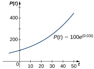
The function [latex]P(t) = 100e^{0.03t}[/latex] models a population starting at 100 individuals with a growth rate of 0.03. This creates the classic J-shaped exponential curve.
Figure 1. An exponential growth model of
We can verify that the function [latex]P(t) = P_0 e^{rt}[/latex] satisfies the initial-value problem:
This differential equation states that the population growth rate is proportional to the current population size, with the constant of proportionality [latex]r[/latex] never changing.
One major problem with exponential growth is its prediction of unlimited population increase. This is unrealistic since various factors limit population growth: birth rate, death rate, food supply, predators, and available space. The growth constant [latex]r[/latex] typically accounts for birth and death rates but ignores these other limiting factors.
Biologists have observed that many populations grow until reaching a steady-state level. This leads to the concept of carrying capacity – the maximum population an environment can sustain indefinitely.
carrying capacity
The maximum population of an organism that an environment can sustain indefinitely. We use the variable [latex]K[/latex] to represent carrying capacity.
The logistic differential equation incorporates carrying capacity to create a more realistic population model:
where [latex]K[/latex] is the carrying capacity, [latex]r[/latex] is the growth rate, and [latex]P(t)[/latex] represents population at time [latex]t[/latex].
logistic differential equation
Let [latex]K[/latex] represent the carrying capacity for a particular organism in a given environment, and let [latex]r[/latex] be a real number that represents the growth rate. The function [latex]P\left(t\right)[/latex] represents the population of this organism as a function of time [latex]t[/latex], and the constant [latex]{P}_{0}[/latex] represents the initial population (population of the organism at time [latex]t=0[/latex]). Then the logistic differential equation is
This equation behaves differently depending on the population size relative to carrying capacity:
When [latex]P[/latex] is small compared to [latex]K[/latex]: The term [latex]\frac{P}{K}[/latex] is close to zero, so [latex]1 - \frac{P}{K} \approx 1[/latex]. The equation becomes approximately [latex]\frac{dP}{dt} = rP[/latex], resembling exponential growth.
As [latex]P[/latex] approaches [latex]K[/latex]: The term [latex]1 - \frac{P}{K}[/latex] gets smaller, slowing the growth rate. When [latex]P = K[/latex], we get [latex]\frac{dP}{dt} = 0[/latex], so population stops changing.
When [latex]P > K[/latex]: The term [latex]1 - \frac{P}{K}[/latex] becomes negative, causing population to decrease toward the carrying capacity.
Populations below carrying capacity grow toward [latex]K[/latex]. Populations above carrying capacity decline toward [latex]K[/latex]. The carrying capacity acts as a stable equilibrium point.
There were an estimated [latex]150[/latex] pileated woodpeckers (Dryocopus pileatus) in a forest at the beginning of 2020. At the beginning of 2021, the population had increased to about [latex]175[/latex]. Based on the size of the forest, the carrying capacity is estimated to be about [latex]400[/latex] pileated woodpeckers.
Write a logistic differential equation and initial condition to model this population. Use [latex]t=0[/latex] for the beginning of 2020.
Draw a direction field for this logistic differential equation, and sketch the solution curve corresponding to the initial condition.
Solve the initial-value problem for [latex]P\left(t\right)[/latex].
According to this model, what will the population be at the beginning of 2025?
How long will it take the population to reach [latex]75%[/latex] of the carrying capacity?
The logistic differential equation formula is [latex]\frac{dP}{dt}=rP \left( 1-\frac{P}{K} \right)[/latex]. We are told that the carrying capacity is [latex]400[/latex] so we substitute this value in for [latex]K[/latex]. To approximate [latex]r[/latex], we can use the fact that the population increased from [latex]150[/latex] to [latex]175[/latex] in one year. Thus, the growth rate is [latex]r = \frac{175-150}{150} = \frac{25}{150} = \frac{1}{6} \approx 16.67%[/latex].To find the initial condition, we use the fact that there are [latex]150[/latex] pileated woodpeckers at the beginning of 2020, so [latex]P_0=150[/latex]. Putting this all together gives us the following initial-value problem.[latex]\frac{dP}{dt}=0.1667 P \left( 1-\frac{P}{400} \right)[/latex], [latex]P\left(0\right)=150[/latex]
We can solve the differential equation using separation of variables.
\begin{array}{rll}
\frac{dP}{dt} & =\hfill 0.1667 P \left( 1-\frac{P}{400} \right) &\hfill \\
\frac{dP}{dt} & =\hfill 0.1667 P \left( \frac{400-P}{400} \right) & \text{Rewrite the expression inside the parentheses}\\
\hfill & \hfill & \text{as one combined fraction.}\\
\frac{dP}{P\left(400-P\right)} & =\hfill\frac{0.1667}{400}dt & \text{Divide both sides by the factors }P\text{ and }400-P\text{.}\\
\hfill & \hfill & \text{Multiply both sides by }dt\text{.}\\
\int \frac{1}{400}\left(\frac{1}{P}-\frac{1}{400-P}\right)dP & =\hfill \int\frac{0.1667}{400}dt & \text{Use partial fraction decomposition to rewrite the left side}\\
\hfill & \hfill & \text{and integrate both sides.}\\
\frac{1}{400}\left( \ln \left| P \right|-\ln \left| 400-P \right|\right) & =\hfill \frac{0.1667}{400}t+C_1 &\hfill\\
\ln \left| \frac{P}{400-P} \right| & =\hfill 0.1667t+C_2 & \text{Multiply both sides by }400\\
\hfill & \hfill & \text{ and use the quotient rule to combine the logarightms.}\\
\left| \frac{P}{400-P} \right| & =\hfill e^{0.1667t+C_2} & \text{Rewrite the equation using the definition of the natural logarithm.}\\
\left| \frac{P}{400-P} \right| & =\hfill C e^{0.1667t} & \text{Rewrite the right side using the properties of exponents.}\\
\frac{P}{400-P} & =\hfill C e^{0.1667t} & \text{If we allow the constant }C\text{ to be positive or negative,}\\
\hfill & \hfill & \text{ we can remove the absolute value.}\\
\end{array}
At this point, we can substitute the values from the initial condition to find [latex]C[/latex].
\begin{array}{rll}
\frac{150}{400-150} \hfill & =\hfill C e^{0.1667 \left( 0 \right)} &&\hfill t=0 \text{ and }P=150\text{.}\\
\frac{150}{250} \hfill & =\hfill C \left( 1 \right) &&\hfill \\
C \hfill & =\hfill \frac{3}{5} &&\hfill
\end{array}
Substitute [latex]C = \frac{3}{5}[/latex] and solve for [latex]P[/latex].
\begin{array}{rll}
\frac{P}{400-P} & =\hfill \frac{3}{5} e^{0.1667t} & \\
P & =\hfill \frac{3}{5} e^{0.1667t} \left( 400-P \right) & \text{Multiply both sides by }400-P\text{.}\\
P & =\hfill 400 \left( \frac{3}{5} \right) e^{0.1667t} – P \left( \frac{3}{5} \right) e^{0.1667t} & \text{Distribute.}\\
P + \frac{3}{5} P e^{0.1667t} & =\hfill240 e^{0.1667t} & \text{Simplify and bring all terms with }P\text{ to the left side.}\\
P \left( 1 + \frac{3}{5} e^{0.1667t} \right) & =\hfill 240 e^{0.1667t} & \text{Factor }P\text{ from the left side.}\\
P & =\hfill \frac{240 e^{0.1667t}}{1 + \frac{3}{5} e^{0.1667t}} & \text{Divide to isolate }P\text{ on the left side.}\\
P \left( t \right) & =\hfill \frac{1200 e^{0.1667t}}{5 + 3 e^{0.1667t}} & \text{Multiply numerator and denominator by }5\text{ to simplify.}
\end{array}
The beginning of 2025 corresponds to [latex]t=5[/latex] and [latex]P \left( 5 \right) \approx 232[/latex]. There will be approximately [latex]232[/latex] pileated woodpeckers at the beginning of 2025.
Note that [latex]75%[/latex] of the carrying capacity is [latex]0.75 \left( 400 \right) = 300[/latex]. We set [latex]P\left(t\right) = 300[/latex] and solve for [latex]t[/latex].
\begin{array}{rll}
\frac{1200 e^{0.1667t}}{5 + 3 e^{0.1667t}} & =\hfill 300 & \\
1200 e^{0.1667t} & =\hfill 300 \left( 5 + 3 e^{0.1667t} \right) & \text{Multiply both sides by the denominator.} \\
1200 e^{0.1667t} & =\hfill 1500 + 900 e^{0.1667t} & \text{Distribute.} \\
300 e^{0.1667t} & =\hfill 1500 & \text{Subtract }900 e^{0.1667t}\text{ from both sides.} \\
t & =\hfill \frac{\ln \left( 5 \right)}{0.1667} & \text{Divide by }300\text{, take the natural logarithm, and divide by }5\text{ on both sides.} \\
t &\approx\hfill 9.65 &
\end{array}
The population will reach [latex]300[/latex] by the end of 2029.