Find integrals when there’s an infinite discontinuity inside your interval
Use the comparison theorem to determine if an improper integral converges
Improper Integrals
Is the area between the graph of [latex]f(x) = \frac{1}{x}[/latex] and the [latex]x[/latex]-axis over the interval [latex][1, +\infty)[/latex] finite or infinite? What about the volume if we revolve this region around the [latex]x[/latex]-axis?
The answer might surprise you: the area is infinite, but the volume is finite. This paradox introduces us to improper integrals—integrals that extend over infinite intervals or involve functions with discontinuities.
improper integrals
Integrals that either have infinite limits of integration or involve functions with discontinuities within the interval of integration.
In this section, we’ll explore how to evaluate these special integrals using limits, discovering when they converge to finite values and when they diverge to infinity.
Integrating over an Infinite Interval
How do we make sense of an integral like [latex]\int_a^{+\infty} f(x) dx[/latex]? We can’t simply plug in infinity as our upper limit.
Instead, we use a limit approach:
First, integrate from [latex]a[/latex] to some finite value [latex]t[/latex]
Then examine what happens as [latex]t[/latex] approaches infinity
Think of it this way: We’re asking “What happens to the area under the curve as we extend our region farther and farther to the right?
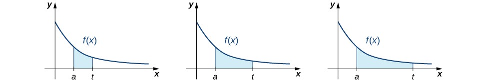
Figure 1 below illustrates this concept. As [latex]t[/latex] increases, the shaded region under [latex]f(x)[/latex] gets wider. The improper integral [latex]\int_a^{+\infty} f(x) dx[/latex] represents the limit of these areas as [latex]t \to +\infty[/latex].
Figure 1. To integrate a function over an infinite interval, we consider the limit of the integral as the upper limit increases without bound.
improper integrals with infinite limits
Type 1: Upper limit approaches [latex]+\infty[/latex]
Let [latex]f(x)[/latex] be continuous over [latex][a, +\infty)[/latex]. Then:
Note: You can split at any point [latex]a[/latex], not just [latex]0[/latex].
[latex]\\[/latex]
Convergence vs. Divergence
Converges: The limit exists and equals a finite number
Diverges: The limit doesn’t exist or approaches [latex]\pm\infty[/latex]
For Type 3 integrals, both parts must converge for the whole integral to converge.
Now let’s tackle the question from our introduction: Is the area between [latex]f(x) = \frac{1}{x}[/latex] and the [latex]x[/latex]-axis over [latex][1, +\infty)[/latex] finite or infinite?
Determine whether the area between the graph of [latex]f\left(x\right)=\frac{1}{x}[/latex] and the x-axis over the interval [latex]\left[1,\text{+}\infty \right)[/latex] is finite or infinite.
We first do a quick sketch of the region in question, as shown in the following graph.
Figure 2. We can find the area between the curve [latex]f\left(x\right)=\frac{1}{x}[/latex] and the x-axis on an infinite interval.
We can see that the area of this region is given by [latex]A={\displaystyle\int }_{1}^{\infty }\frac{1}{x}dx[/latex]. Then we have
[latex]\begin{array}{ccccc}\hfill A& ={\displaystyle\int }_{1}^{\infty }\frac{1}{x}dx\hfill & & & \\ & =\underset{t\to \text{+}\infty }{\text{lim}}{\displaystyle\int }_{1}^{t}\frac{1}{x}dx\hfill & & & \text{Rewrite the improper integral as a limit.}\hfill \\ & =\underset{t\to \text{+}\infty }{\text{lim}}\text{ln}|x||{}_{\begin{array}{c}\\ 1\end{array}}^{\begin{array}{c}t\\ \end{array}}\hfill & & & \text{Find the antiderivative.}\hfill \\ & =\underset{t\to \text{+}\infty }{\text{lim}}\left(\text{ln}|t|-\text{ln}1\right)\hfill & & & \text{Evaluate the antiderivative.}\hfill \\ & =\text{+}\infty .\hfill & & & \text{Evaluate the limit.}\hfill \end{array}[/latex]
Since the improper integral diverges to [latex]+\infty[/latex], the area of the region is infinite.
Find the volume of the solid obtained by revolving the region bounded by the graph of [latex]f\left(x\right)=\frac{1}{x}[/latex] and the x-axis over the interval [latex]\left[1,\text{+}\infty \right)[/latex] about the [latex]x[/latex] -axis.
The solid is shown in Figure 3. Using the disk method, we see that the volume V is
The improper integral converges to [latex]\pi[/latex]. Therefore, the volume of the solid of revolution is [latex]\pi[/latex].
In conclusion, although the area of the region between the [latex]x[/latex]-axis and the graph of [latex]f\left(x\right)=\frac{1}{x}[/latex] over the interval [latex]\left[1,\text{+}\infty \right)[/latex] is infinite, the volume of the solid generated by revolving this region about the [latex]x[/latex]-axis is finite. The solid generated is known as Gabriel’s Horn.
Because improper integrals require evaluating limits at infinity, at times we may be required to use L’Hôpital’s Rule to evaluate a limit.
Recall: L’Hôpital’s Rule
Suppose [latex]f[/latex] and [latex]g[/latex] are differentiable functions over an open interval [latex]\left(a, \infty \right)[/latex] for some value of [latex]a[/latex]. If either:
[latex]\underset{x\to \infty}{\lim}f(x)=0[/latex] and [latex]\underset{x\to \infty}{\lim}g(x)=0[/latex]
[latex]\underset{x\to \infty}{\lim}f(x)= \infty[/latex] (or [latex]-\infty[/latex]) and [latex]\underset{x\to \infty}{\lim}g(x)= \infty[/latex] (or [latex]-\infty[/latex]), then
If either [latex]{\displaystyle\int }_{\text{-}\infty }^{0}x{e}^{x}dx[/latex] or [latex]{\displaystyle\int }_{0}^{+\infty }x{e}^{x}dx[/latex] diverges, then [latex]{\displaystyle\int }_{\text{-}\infty }^{+\infty }x{e}^{x}dx[/latex] diverges. Compute each integral separately. For the first integral,
[latex]\begin{array}{ccccc}\hfill {\displaystyle\int _{-\infty }^{0}x{e}^{x}dx}& ={\underset{t\to -\infty}\lim}{\displaystyle\int _{t}^{0}x{e}^{x}dx}\hfill & & & \text{Rewrite as a limit.}\hfill \\ & ={\underset{t\to -\infty}\lim}\left(x{e}^{x}-{e}^{x}\right)\Biggr|_{t}^{0} \hfill & & & \begin{array}{c}\text{Use integration by parts to find the} \hfill \\ \text{antiderivative. (Here } u=x \text{ and } dv=e_{dv}^{x}\text{.)}\end{array} \\ & ={\underset{t\to -\infty}\lim}\left(-1-t{e}^{t}+{e}^{t}\right)\hfill & & & \text{Evaluate the antiderivative.}\hfill \\ & =-1.\hfill & & & \begin{array}{c}\text{Evaluate the limit.}\mathit{\text{Note:}} {\underset{t\to -\infty}\lim}t{e}^{t}\text{is}\hfill \\ \text{indeterminate of the form}0\cdot \infty .\text{Thus,}\hfill \\ {\underset{t\to -\infty}\lim}t{e}^{t}={\underset{t\to -\infty}\lim}\frac{t}{{e}^{\text{-}t}}={\underset{t\to -\infty}\lim}\frac{-1}{{e}^{-t}}={\underset{t\to -\infty}\lim}-{e}^{t}=0\text{by}\hfill \\ \text{L'H}\hat{o}\text{pital's Rule.}\hfill \end{array}\hfill \end{array}[/latex]
The first improper integral converges. For the second integral,
Thus, [latex]{\displaystyle\int }_{0}^{+\infty }x{e}^{x}dx[/latex] diverges. Since this integral diverges, [latex]{\displaystyle\int }_{\text{-}\infty }^{+\infty }x{e}^{x}dx[/latex] diverges as well.