Just as we analyze symmetry in rectangular coordinates to understand function behavior, we can examine symmetry in polar curves to reveal important properties and simplify graphing.
Symmetry in Rectangular Coordinates:
Even functions: [latex]f(-x) = f(x)[/latex] creates [latex]y[/latex]-axis symmetry
Polar curves exhibit three main types of symmetry, each corresponding to reflection across a different line or point.
symmetry in polar curves and equations
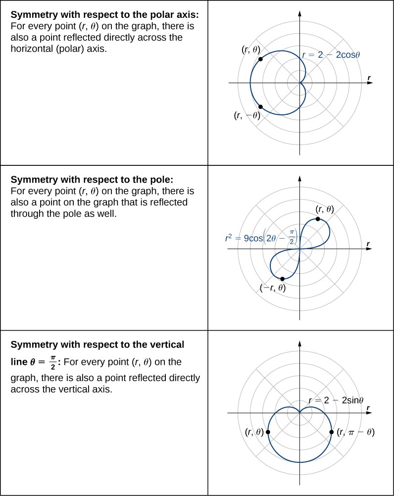
For a curve [latex]r=f\left(\theta \right)[/latex] in polar coordinates, we can test for three types of symmetry:
Polar Axis Symmetry (horizontal line symmetry)
If point [latex]\left(r,\theta \right)[/latex] is on the graph, then [latex]\left(r,-\theta \right)[/latex] is also on the graph
Test: Replace [latex]\theta[/latex] with [latex]-\theta[/latex] in the equation
Pole Symmetry (origin symmetry)
If point [latex]\left(r,\theta \right)[/latex] is on the graph, then [latex](r,\pi + \theta)[/latex] is also on the graph
Test: Replace [latex]r[/latex] with [latex]-r[/latex], or replace [latex]\theta[/latex] with [latex]\pi + \theta[/latex]
Vertical Line Symmetry (line [latex]\theta = \frac{\pi}{2}[/latex])
If point [latex]\left(r,\theta \right)[/latex] is on the graph, then [latex](r,\pi - \theta)[/latex] is also on the graph
Test: Replace [latex]\theta[/latex] with [latex]\pi - \theta[/latex] in the equation
Understanding these symmetries helps you graph polar curves more efficiently. If you can establish that a curve has certain symmetries, you only need to plot points in one region and then reflect them to complete the entire graph.
The following table shows examples of each type of symmetry.
Figure 11.
Find the symmetry of the rose defined by the equation [latex]r=3\sin\left(2\theta \right)[/latex] and create a graph.
Suppose the point [latex]\left(r,\theta \right)[/latex] is on the graph of [latex]r=3\sin\left(2\theta \right)[/latex].
To test for symmetry about the polar axis, first try replacing [latex]\theta[/latex] with [latex]-\theta[/latex]. This gives [latex]r=3\sin\left(2\left(-\theta \right)\right)=-3\sin\left(2\theta \right)[/latex]. Since this changes the original equation, this test is not satisfied. However, returning to the original equation and replacing [latex]r[/latex] with [latex]-r[/latex] and [latex]\theta[/latex] with [latex]\pi -\theta[/latex] yields
Multiplying both sides of this equation by [latex]-1[/latex] gives [latex]r=3\sin2\theta[/latex], which is the original equation. This demonstrates that the graph is symmetric with respect to the polar axis.
To test for symmetry with respect to the pole, first replace [latex]r[/latex] with [latex]-r[/latex], which yields [latex]-r=3\sin\left(2\theta \right)[/latex]. Multiplying both sides by −1 gives [latex]r=-3\sin\left(2\theta \right)[/latex], which does not agree with the original equation. Therefore the equation does not pass the test for this symmetry. However, returning to the original equation and replacing [latex]\theta[/latex] with [latex]\theta +\pi[/latex] gives
Since this agrees with the original equation, the graph is symmetric about the pole.
To test for symmetry with respect to the vertical line [latex]\theta =\frac{\pi }{2}[/latex], first replace both [latex]r[/latex] with [latex]-r[/latex] and [latex]\theta[/latex] with [latex]-\theta[/latex].
Multiplying both sides of this equation by [latex]-1[/latex] gives [latex]r=3\sin2\theta[/latex], which is the original equation. Therefore the graph is symmetric about the vertical line [latex]\theta =\frac{\pi }{2}[/latex].
This graph has symmetry with respect to the polar axis, the origin, and the vertical line going through the pole. To graph the function, tabulate values of [latex]\theta[/latex] between 0 and [latex]\frac{\pi}{2}[/latex] and then reflect the resulting graph.
[latex]\theta[/latex]
[latex]r[/latex]
[latex]0[/latex]
[latex]0[/latex]
[latex]\frac{\pi }{6}[/latex]
[latex]\frac{3\sqrt{3}}{2}\approx 2.6[/latex]
[latex]\frac{\pi }{4}[/latex]
[latex]3[/latex]
[latex]\frac{\pi }{3}[/latex]
[latex]\frac{3\sqrt{3}}{2}\approx 2.6[/latex]
[latex]\frac{\pi }{2}[/latex]
[latex]0[/latex]
This gives one petal of the rose, as shown in the following graph.
Figure 12. The graph of the equation between [latex]\theta =0[/latex] and [latex]\theta =\frac{\pi}{2}[/latex].
Reflecting this image into the other three quadrants gives the entire graph as shown.
Figure 13. The entire graph of the equation is called a four-petaled rose.
Watch the following video to see the worked solution to the example above.
For closed captioning, open the video on its original page by clicking the Youtube logo in the lower right-hand corner of the video display. In YouTube, the video will begin at the same starting point as this clip, but will continue playing until the very end.