- Determine the volume of a solid formed by rotating a region around an axis using cylindrical shells
- Evaluate the benefits and limitations of different methods (disk, washer, cylindrical shells) for calculating volumes
Cylindrical Shells Method
Let’s explore the final method for finding the volume of a solid of revolution—the method of cylindrical shells. This method can be used on the same types of solids as the disk or washer method; however, we integrate along the coordinate axis parallel to the axis of revolution. This ability to choose which variable of integration to use can be a significant advantage with more complicated functions. Additionally, the specific geometry of the solid sometimes makes the method of using cylindrical shells more appealing than the washer method.
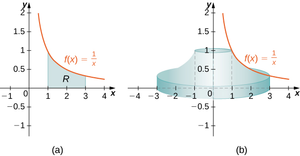
Again, we are working with a solid of revolution. We define a region [latex]R,[/latex] bounded above by the graph of a function [latex]y=f(x),[/latex] below by the [latex]x[/latex]-axis, and on the left and right by the lines [latex]x=a[/latex] and [latex]x=b,[/latex] respectively, as shown in Figure 1(a). We then revolve this region around the [latex]y[/latex]-axis, as shown in Figure 1(b).
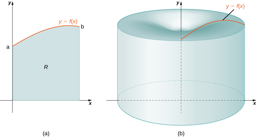
Note that this is different from what we have done before. Previously, regions defined in terms of functions of [latex]x[/latex] were revolved around the [latex]x[/latex]-axis or a line parallel to it.
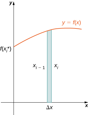
Next, as we have done many times before, partition the interval [latex]\left[a,b\right][/latex] using a regular partition, [latex]P=\left\{{x}_{0},{x}_{1}\text{,…},{x}_{n}\right\}[/latex] and, for [latex]i=1,2\text{,…},n,[/latex] choose a point [latex]{x}_{i}^{*}\in \left[{x}_{i-1},{x}_{i}\right].[/latex]
Then, construct a rectangle over the interval [latex]\left[{x}_{i-1},{x}_{i}\right][/latex] of height [latex]f({x}_{i}^{*})[/latex] and width [latex]\text{Δ}x.[/latex]
When that rectangle is revolved around the [latex]y[/latex]-axis, instead of a disk or a washer, we get a cylindrical shell, as shown in the following figure.
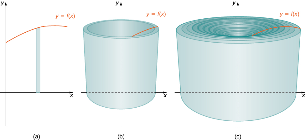
To calculate the volume of this shell, consider the following.
Notice that the rectangle we are using is parallel to the axis of revolution (y axis), not perpendicular like the disk and washer method. This could be very useful, particularly for [latex]y[/latex]-axis revolutions.
The shell is a cylinder, so its volume is the cross-sectional area multiplied by the height of the cylinder. The cross-sections are annuli (ring-shaped regions—essentially, circles with a hole in the center), with outer radius [latex]{x}_{i}[/latex] and inner radius [latex]{x}_{i-1}.[/latex]
Thus, the cross-sectional area is [latex]\pi {x}_{i}^{2}-\pi {x}_{i-1}^{2}.[/latex] The height of the cylinder is [latex]f({x}_{i}^{*}).[/latex]
Then the volume of the shell is:
Note that [latex]{x}_{i}-{x}_{i-1}=\text{Δ}x,[/latex] so we have:
Furthermore, [latex]\frac{{x}_{i}+{x}_{i-1}}{2}[/latex] is both the midpoint of the interval [latex]\left[{x}_{i-1},{x}_{i}\right][/latex] and the average radius of the shell, and we can approximate this by [latex]{x}_{i}^{*}.[/latex]
We then have:
Another way to think of this is to think of making a vertical cut in the shell and then opening it up to form a flat plate (Figure 4).
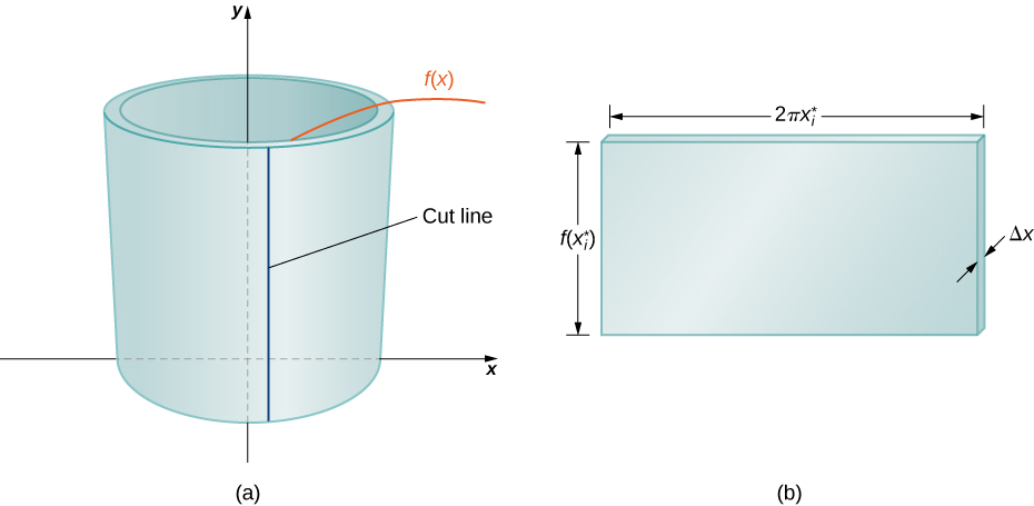
In reality, the outer radius of the shell is greater than the inner radius, and hence the back edge of the plate would be slightly longer than the front edge of the plate. However, we can approximate the flattened shell by a flat plate of height [latex]f({x}_{i}^{*}),[/latex] width [latex]2\pi {x}_{i}^{*},[/latex] and thickness [latex]\text{Δ}x[/latex] (Figure 4).
The volume of the shell, then, is approximately the volume of the flat plate. Multiplying the height, width, and depth of the plate, we get:
which is the same formula we had before.
To calculate the volume of the entire solid, we then add the volumes of all the shells and obtain:
Here we have another Riemann sum, this time for the function [latex]2\pi xf(x).[/latex] Taking the limit as [latex]n\to \infty[/latex] gives us:
This leads to the following rule for the method of cylindrical shells.
the method of cylindrical shells
Let [latex]f(x)[/latex] be continuous and nonnegative.
Define [latex]R[/latex] as the region bounded above by the graph of [latex]f(x),[/latex] below by the [latex]x\text{-axis},[/latex] on the left by the line [latex]x=a,[/latex] and on the right by the line [latex]x=b.[/latex]
Then the volume of the solid of revolution formed by revolving [latex]R[/latex] around the [latex]y[/latex]-axis is given by:
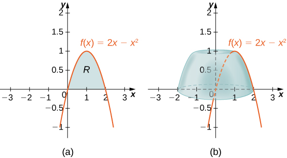
Define [latex]R[/latex] as the region bounded above by the graph of [latex]f(x)=1\text{/}x[/latex] and below by the [latex]x\text{-axis}[/latex] over the interval [latex]\left[1,3\right].[/latex] Find the volume of the solid of revolution formed by revolving [latex]R[/latex] around the [latex]y\text{-axis}.[/latex]
Define [latex]R[/latex] as the region bounded above by the graph of [latex]f(x)=2x-{x}^{2}[/latex] and below by the [latex]x\text{-axis}[/latex] over the interval [latex]\left[0,2\right].[/latex] Find the volume of the solid of revolution formed by revolving [latex]R[/latex] around the [latex]y\text{-axis}.[/latex]