Understanding Limits: Get Stronger

Lumen Learning

Understanding Limits: Get Stronger

A Preview of Calculus

For the following exercises (1-3), points $P(1,2)$ and $Q(x,y)$ are on the graph of the function $f(x)=x^2+1$ .

Complete the following table with the appropriate values: $y$ -coordinate of Q, the point $Q(x,y),$ and the slope of the secant line passing through points P and Q. Round your answer to eight significant digits.

$x$ $y$ $Q(x,y)$ $m_{\sec}$

$1.1$ a. e. i.

$1.01$ b. f. j.

$1.001$ c. g. k.

$1.0001$ d. h. l.
Use the values in the right column of the table in the preceding exercise to guess the value of the slope of the line tangent to $f$ at $x=1$ .
Use the value in the preceding exercise to find the equation of the tangent line at point $P$ . Graph $f(x)$ and the tangent line.

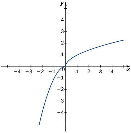
For the following exercises (4-6), points $P(1,1)$ and $Q(x,y)$ are on the graph of the function $f(x)=x^3$ .

Complete the following table with the appropriate values: $y$ -coordinate of $Q$ , the point $Q(x,y)$ , and the slope of the secant line passing through points $P$ and $Q$ . Round your answer to eight significant digits.

$x$ $y$ $Q(x,y)$ $m_{\sec}$

$1.1$ a. e. i.

$1.01$ b. f. j.

$1.001$ c. g. k.

$1.0001$ d. h. l.
Use the values in the right column of the table in the preceding exercise to guess the value of the slope of the tangent line to $f$ at $x=1$ .
Use the value in the preceding exercise to find the equation of the tangent line at point $P$ . Graph $f(x)$ and the tangent line.

For the following exercises (7-9), points $P(4,2)$ and $Q(x,y)$ are on the graph of the function $f(x)=\sqrt{x}$ .

Complete the following table with the appropriate values: $y$ -coordinate of $Q$ , the point $Q(x,y)$ , and the slope of the secant line passing through points $P$ and $Q$ . Round your answer to eight significant digits.

$x$ $y$ $Q(x,y)$ $m_{\sec}$

$4.1$ a. e. i.

$4.01$ b. f. j.

$4.001$ c. g. k.

$4.0001$ d. h. l.
Use the values in the right column of the table in the preceding exercise to guess the value of the slope of the tangent line to $f$ at $x=4$ .
Use the value in the preceding exercise to find the equation of the tangent line at point $P$ .

For the following exercises (10-12), points $P(1.5,0)$ and $Q(\phi ,y)$ are on the graph of the function $f(\phi )= \cos (\pi \phi )$ .

Complete the following table with the appropriate values: $y$ -coordinate of $Q$ , the point $Q(x,y)$ , and the slope of the secant line passing through points $P$ and $Q$ . Round your answer to eight significant digits.

$x$ $y$ $Q(\phi ,y)$ $m_{\sec}$

$1.4$ a. e. i.

$1.49$ b. f. j.

$1.499$ c. g. k.

$1.4999$ d. h. l.
Use the values in the right column of the table in the preceding exercise to guess the value of the slope of the tangent line to $f$ at $x=4$ .
Use the value in the preceding exercise to find the equation of the tangent line at point $P$ .

For the following exercises (13-15), points $P(-1,-1)$ and $Q(x,y)$ are on the graph of the function $f(x)=\dfrac{1}{x}$ .

Complete the following table with the appropriate values: $y$ -coordinate of $Q$ , the point $Q(x,y)$ , and the slope of the secant line passing through points $P$ and $Q$ . Round your answer to eight significant digits.

$x$ $y$ $Q(x,y)$ $m_{\sec}$

$-1.05$ a. e. i.

$-1.01$ b. f. j.

− $-1.005$ c. g. k.

$-1.001$ d. h. l.
Use the values in the right column of the table in the preceding exercise to guess the value of the slope of the line tangent to $f$ at $x=-1$ .
Use the value in the preceding exercise to find the equation of the tangent line at point $P$ .

For the following exercises (16-17), the position function of a ball dropped from the top of a 200-meter tall building is given by $s(t)=200-4.9t^2$ , where position $s$ is measured in meters and time $t$ is measured in seconds. Round your answer to eight significant digits.

Compute the average velocity of the ball over the given time intervals.
1. $[4.99,5]$
2. $[5,5.01]$
3. $[4.999,5]$
4. $[5,5.001]$
Use the preceding exercise to guess the instantaneous velocity of the ball at $t=5$ sec.

For the following exercises (18-19), consider a stone tossed into the air from ground level with an initial velocity of 15 m/sec. Its height in meters at time $t$ seconds is $h(t)=15t-4.9t^2$ .

Compute the average velocity of the stone over the given time intervals.
1. $[1,1.05]$
2. $[1,1.01]$
3. $[1,1.005]$
4. $[1,1.001]$
Use the preceding exercise to guess the instantaneous velocity of the stone at $t=1$ sec.

For the following exercises (20-21), consider a rocket shot into the air that then returns to Earth. The height of the rocket in meters is given by $h(t)=600+78.4t-4.9t^2$ , where $t$ is measured in seconds.

Compute the average velocity of the rocket over the given time intervals.
1. $[9,9.01]$
2. $[8.99,9]$
3. $[9,9.001]$
4. $[8.999,9]$
Use the preceding exercise to guess the instantaneous velocity of the rocket at $t=9$ sec.

For the following exercises (22-23), consider an athlete running a 40-m dash. The position of the athlete is given by $d(t)=\dfrac{t^3}{6}+4t$ , where $d$ is the position in meters and $t$ is the time elapsed, measured in seconds.

Compute the average velocity of the runner over the given time intervals.
1. $[1.95,2.05]$
2. $[1.995,2.005]$
3. $[1.9995,2.0005]$
4. $[2,2.00001]$
Use the preceding exercise to guess the instantaneous velocity of the runner at $t=2$ sec.

For the following exercises (24-25), consider the function $f(x)=|x|$ .

Sketch the graph of $f$ over the interval $[-1,2]$ and shade the region above the $x$ -axis.
Use the preceding exercise to find the exact value of the area between the $x$ -axis and the graph of $f$ over the interval $[-1,2]$ using rectangles. For the rectangles, use the square units, and approximate both above and below the lines. Use geometry to find the exact answer.

For the following exercises (26-27), consider the function $f(x)=\sqrt{1-x^2}$ . (Hint: This is the upper half of a circle of radius $1$ positioned at $(0,0)$ .)

Sketch the graph of $f$ over the interval $[-1,1]$ .
Use the preceding exercise to find the exact area between the $x$ -axis and the graph of $f$ over the interval $[-1,1]$ using rectangles. For the rectangles, use squares [/latex]0.4[/latex] by $0.4$ units, and approximate both above and below the lines. Use geometry to find the exact answer.

For the following exercises (28-29), consider the function $f(x)=−x^2+1$ .

Sketch the graph of $f$ over the interval $[-1,1]$ .
Approximate the area of the region between the $x$ -axis and the graph of $f$ over the interval $[-1,1]$ .

Introduction to the limit of a function

In the following exercises (1-3), set up a table of values to find the indicated limit. Round to eight digits.

$\underset{x\to 1}{\lim}(1-2x)$

$x$ $1-2x$ $x$ $1-2x$

0.9 a. $1.1$ e.

0.99 b. $1.01$ f.

0.999 c. $1.001$ g.

0.9999 d. $1.0001$ h.

$\underset{z\to 0}{\lim}\dfrac{z-1}{z^2(z+3)}$

$z$	$\frac{z-1}{z^2(z+3)}$	$z$	$\frac{z-1}{z^2(z+3)}$
$−0.1$	a.	$0.1$	e.
$−0.01$	b.	$0.01$	f.
$−0.001$	c.	$0.001$	g.
$−0.0001$	d.	$0.0001$	h.

$\underset{x\to 2^-}{\lim}\dfrac{1-\frac{2}{x}}{x^2-4}$

$x$	$\frac{1-\frac{2}{x}}{x^2-4}$	$x$	$\frac{1-\frac{2}{x}}{x^2-4}$
$1.9$	a.	$2.1$	e.
$1.99$	b.	$2.01$	f.
$1.999$	c.	$2.001$	g.
$1.9999$	d.	$2.0001$	h.

In the following exercise, set up a table of values and round to eight significant digits. Based on the table of values, make a guess about what the limit is. Then, use a calculator to graph the function and determine the limit. Was the conjecture correct? If not, why does the method of tables fail?

$\underset{\alpha \to 0^+}{\lim}\frac{1}{\alpha} \cos \left(\frac{\pi }{\alpha }\right)$

$a$ $\frac{1}{\alpha } \cos (\frac{\pi }{\alpha })$

$0.1$ a.

$0.01$ b.

$0.001$ c.

$0.0001$ d.

In the following exercises (5-6), consider the graph of the function $y=f(x)$ shown here. Which of the statements about $y=f(x)$ are true and which are false? Explain why a statement is false.

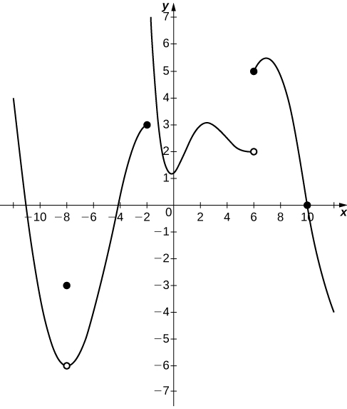
$\underset{x\to -2^+}{\lim}f(x)=3$
$\underset{x\to 6}{\lim}f(x)=5$

In the following exercises (7-9), use the following graph of the function $y=f(x)$ to find the values, if possible. Estimate when necessary.

A graph of a piecewise function with two segments. The first segment exists for x <=1, and the second segment exists for x > 1. The first segment is linear with a slope of 1 and goes through the origin. Its endpoint is a closed circle at (1,1). The second segment is also linear with a slope of -1. It begins with the open circle at (1,2).

$\underset{x\to 1^-}{\lim}f(x)$
$\underset{x\to 1^+}{\lim}f(x)$
$\underset{x\to 1}{\lim}f(x)$

In the following exercises 10-11), use the graph of the function $y=f(x)$ shown here to find the values, if possible. Estimate when necessary.

A graph of a piecewise function with two segments. The first is a linear function for x < 0. There is an open circle at (0,1), and its slope is -1. The second segment is the right half of a parabola opening upward. Its vertex is a closed circle at (0, -4), and it goes through the point (2,0).

$\underset{x\to 0^-}{\lim}f(x)$
$\underset{x\to 0}{\lim}f(x)$

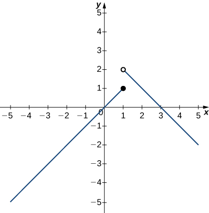
In the following exercises (12-17), use the graph of the function $y=f(x)$ shown here to find the values, if possible. Estimate when necessary.

A graph of a piecewise function with three segments, all linear. The first exists for x < -2, has a slope of 1, and ends at the open circle at (-2, 0). The second exists over the interval [-2, 2], has a slope of -1, goes through the origin, and has closed circles at its endpoints (-2, 2) and (2,-2). The third exists for x>2, has a slope of 1, and begins at the open circle (2,2).

$\underset{x\to -2^-}{\lim}f(x)$
$\underset{x\to -2^+}{\lim}f(x)$
$\underset{x\to -2}{\lim}f(x)$
$\underset{x\to 2^-}{\lim}f(x)$
$\underset{x\to 2^+}{\lim}f(x)$
$\underset{x\to 2}{\lim}f(x)$

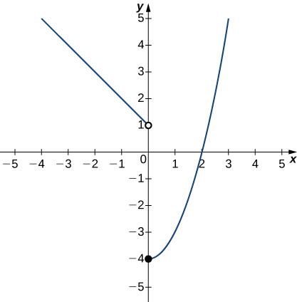
In the following exercises (18-20), use the graph of the function $y=g(x)$ shown here to find the values, if possible. Estimate when necessary.

A graph of a piecewise function with two segments. The first exists for x>=0 and is the left half of an upward opening parabola with vertex at the closed circle (0,3). The second exists for x>0 and is the right half of a downward opening parabola with vertex at the open circle (0,0).

$\underset{x\to 0^-}{\lim}g(x)$
$\underset{x\to 0^+}{\lim}g(x)$
$\underset{x\to 0}{\lim}g(x)$

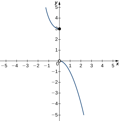
In the following exercises (21-23), use the graph of the function $y=h(x)$ shown here to find the values, if possible. Estimate when necessary.

A graph of a function with two curves approaching 0 from quadrant 1 and quadrant 3. The curve in quadrant one appears to be the top half of a parabola opening to the right of the y axis along the x axis with vertex at the origin. The curve in quadrant three appears to be the left half of a parabola opening downward with vertex at the origin.

$\underset{x\to 0^-}{\lim}h(x)$
$\underset{x\to 0^+}{\lim}h(x)$
$\underset{x\to 0}{\lim}h(x)$

In the following exercises (24-25), sketch the graph of a function with the given properties.

$\underset{x\to -\infty }{\lim}f(x)=0, \, \underset{x\to -1^-}{\lim}f(x)=−\infty$ , $\underset{x\to -1^+}{\lim}f(x)=\infty, \, \underset{x\to 0}{\lim}f(x)=f(0), \, f(0)=1, \, \underset{x\to \infty }{\lim}f(x)=−\infty$
$\underset{x\to -\infty }{\lim}f(x)=2, \, \underset{x\to -2}{\lim}f(x)=−\infty$ , $\underset{x\to \infty }{\lim}f(x)=2, \, f(0)=0$

$x$	$1-2x$	$x$	$1-2x$
0.9	a.	$1.1$	e.
0.99	b.	$1.01$	f.
0.999	c.	$1.001$	g.
0.9999	d.	$1.0001$	h.

$x$	$y$	$Q(x,y)$	$m_{\sec}$
$4.1$	a.	e.	i.
$4.01$	b.	f.	j.
$4.001$	c.	g.	k.
$4.0001$	d.	h.	l.

$x$	$y$	$Q(\phi ,y)$	$m_{\sec}$
$1.4$	a.	e.	i.
$1.49$	b.	f.	j.
$1.499$	c.	g.	k.
$1.4999$	d.	h.	l.

$x$	$y$	$Q(x,y)$	$m_{\sec}$
$-1.05$	a.	e.	i.
$-1.01$	b.	f.	j.
− $-1.005$	c.	g.	k.
$-1.001$	d.	h.	l.

$a$	$\frac{1}{\alpha } \cos (\frac{\pi }{\alpha })$
$0.1$	a.
$0.01$	b.
$0.001$	c.
$0.0001$	d.