Trigonometric Functions: Learn It 4

Graphs and Periods of the Trigonometric Functions

We have seen that as we travel around the unit circle, the values of the trigonometric functions repeat. This repetition is evident in the functions’ graphs, showcasing their periodic nature. For any angle [latex]\theta[/latex] on the unit circle, the function values at [latex]\theta[/latex] and [latex]\theta +2\pi[/latex] are identical, since these angles correspond to the same point. Consequently, the trigonometric functions are periodic functions.

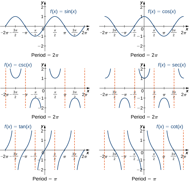
The sine, cosine, secant, and cosecant functions have a period of [latex]2\pi[/latex]. Since the tangent and cotangent functions repeat on an interval of length [latex]\pi[/latex], their period is [latex]\pi[/latex] (Figure 9).

periods of the trigonometric functions

Trigonometric functions are periodic, meaning they repeat their values over specific intervals.

Sine, cosine, and secant have a period of [latex]2\pi[/latex] radians, while tangent and cotangent have a period of [latex]\pi[/latex] radians.


An image of six graphs. Each graph has an x axis that runs from -2 pi to 2 pi and a y axis that runs from -2 to 2. The first graph is of the function “f(x) = sin(x)”, which is a curved wave function. The graph of the function starts at the point (-2 pi, 0) and increases until the point (-((3 pi)/2), 1). After this point, the function decreases until the point (-(pi/2), -1). After this point, the function increases until the point ((pi/2), 1). After this point, the function decreases until the point (((3 pi)/2), -1). After this point, the function begins to increase again. The x intercepts shown on the graph are at the points (-2 pi, 0), (-pi, 0), (0, 0), (pi, 0), and (2 pi, 0). The y intercept is at the origin. The second graph is of the function “f(x) = cos(x)”, which is a curved wave function. The graph of the function starts at the point (-2 pi, 1) and decreases until the point (-pi, -1). After this point, the function increases until the point (0, 1). After this point, the function decreases until the point (pi, -1). After this point, the function increases again. The x intercepts shown on the graph are at the points (-((3 pi)/2), 0), (-(pi/2), 0), ((pi/2), 0), and (((3 pi)/2), 0). The y intercept is at the point (0, 1). The graph of cos(x) is the same as the graph of sin(x), except it is shifted to the left by a distance of (pi/2). On the next four graphs there are dotted vertical lines which are not a part of the function, but act as boundaries for the function, boundaries the function will never touch. They are known as vertical asymptotes. There are infinite vertical asymptotes for all of these functions, but these graphs only show a few. The third graph is of the function “f(x) = csc(x)”. The vertical asymptotes for “f(x) = csc(x)” on this graph occur at “x = -2 pi”, “x = -pi”, “x = 0”, “x = pi”, and “x = 2 pi”. Between the “x = -2 pi” and “x = -pi” asymptotes, the function looks like an upward facing “U”, with a minimum at the point (-((3 pi)/2), 1). Between the “x = -pi” and “x = 0” asymptotes, the function looks like an downward facing “U”, with a maximum at the point (-(pi/2), -1). Between the “x = 0” and “x = pi” asymptotes, the function looks like an upward facing “U”, with a minimum at the point ((pi/2), 1). Between the “x = pi” and “x = 2 pi” asymptotes, the function looks like an downward facing “U”, with a maximum at the point (((3 pi)/2), -1). The fourth graph is of the function “f(x) = sec(x)”. The vertical asymptotes for this function on this graph are at “x = -((3 pi)/2)”, “x = -(pi/2)”, “x = (pi/2)”, and “x = ((3 pi)/2)”. Between the “x = -((3 pi)/2)” and “x = -(pi/2)” asymptotes, the function looks like an downward facing “U”, with a maximum at the point (-pi, -1). Between the “x = -(pi/2)” and “x = (pi/2)” asymptotes, the function looks like an upward facing “U”, with a minimum at the point (0, 1). Between the “x = (pi/2)” and “x = (3pi/2)” asymptotes, the function looks like an downward facing “U”, with a maximum at the point (pi, -1). The graph of sec(x) is the same as the graph of csc(x), except it is shifted to the left by a distance of (pi/2). The fifth graph is of the function “f(x) = tan(x)”. The vertical asymptotes of this function on this graph occur at “x = -((3 pi)/2)”, “x = -(pi/2)”, “x = (pi/2)”, and “x = ((3 pi)/2)”. In between all of the vertical asymptotes, the function is always increasing but it never touches the asymptotes. The x intercepts on this graph occur at the points (-2 pi, 0), (-pi, 0), (0, 0), (pi, 0), and (2 pi, 0). The y intercept is at the origin. The sixth graph is of the function “f(x) = cot(x)”. The vertical asymptotes of this function on this graph occur at “x = -2 pi”, “x = -pi”, “x = 0”, “x = pi”, and “x = 2 pi”. In between all of the vertical asymptotes, the function is always decreasing but it never touches the asymptotes. The x intercepts on this graph occur at the points (-((3 pi)/2), 0), (-(pi/2), 0), ((pi/2), 0), and (((3 pi)/2), 0) and there is no y intercept.
Figure 9. The six trigonometric functions are periodic.

Transformations to Trigonometric Graphs

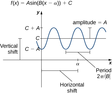
Just as with algebraic functions, we can apply transformations to trigonometric functions. Transforming a trigonometric function like

[latex]f(x)=A \sin(B(x-\alpha))+C[/latex]
adjusts its shape and position on a graph.

In this equation, the constant [latex]A[/latex] affects the amplitude or height of the wave, [latex]B[/latex] impacts the period or width of each cycle, [latex]\alpha[/latex] controls the horizontal shift, and [latex]C[/latex] shifts the graph up or down vertically.

An image of a graph. The graph is of the function “f(x) = Asin(B(x - alpha)) + C”. Along the y axis, there are 3 hash marks: starting from the bottom and moving up, the hash marks are at the values “C - A”, “C”, and “C + A”. The distance from the origin to “C” is labeled “vertical shift”. The distance from “C - A” to “A” and the distance from “A” to “C + A” is “A”, which is labeled “amplitude”. On the x axis is a hash mark at the value “alpha” and the distance between the origin and “alpha” is labeled “horizontal shift”. The distance between two successive minimum values of the function (in other words, the distance between two bottom parts of the wave that are next to each other) is “(2 pi)/(absolute value of B)” is labeled the period. The period is also the distance between two successive maximum values of the function.
Figure 10. A graph of a general sine function.

Breaking Down Trigonometric Transformations

  1. Amplitude Adjustment: Multiply the function by [latex]A[/latex] to stretch or compress it vertically. If [latex]A[/latex] is greater than [latex]1[/latex], the function stretches; if [latex]A[/latex] is between [latex]0[/latex] and [latex]1[/latex], it compresses.
  2. Period Modification: Multiply the input variable by [latex]B[/latex]. If [latex]B[/latex] is greater than [latex]1[/latex], the function’s period decreases, leading to more cycles in the same space. If [latex]B[/latex] is between [latex]0[/latex] and [latex]1[/latex], the period increases, and the function stretches horizontally.
  3. Horizontal Shift: Subtract [latex]\alpha[/latex] from the input variable to shift the graph horizontally. If [latex]\alpha[/latex] is positive, the shift is to the right; if negative, to the left.
  4. Vertical Shift: Add [latex]C[/latex] to the function to move the graph up or down. If [latex]C[/latex] is positive, the graph shifts upwards; if negative, it shifts downwards.

The transformations applied to the sine function can similarly be applied to the cosine function. In the general form of a cosine function [latex]f(x)=A \cos(B(x-\alpha))+C[/latex], the constants [latex]A[/latex], [latex]B[/latex], [latex]\alpha[/latex], and [latex]C[/latex] cause the same types of transformations as they do with the sine function.

Describe the relationship between the graph of [latex]f(x)=3\sin(4x)-5[/latex] and the graph of [latex]y=\sin x[/latex].

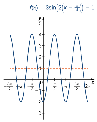
Sketch a graph of [latex]f(x)=3\sin(2(x-\frac{\pi}{4}))+1[/latex].