The Mean Value Theorem: Learn It 2

Lumen Learning

The Mean Value Theorem: Learn It 2

Use Rolle’s theorem and the Mean Value Theorem to show how functions behave between two points
Discuss three key implications of the Mean Value Theorem for understanding function behavior

The Mean Value Theorem

The Mean Value Theorem is one of the most important theorems in calculus. We look at some of its implications at the end of this section. First, let’s start with a special case of the Mean Value Theorem, called Rolle’s theorem.

Rolle’s Theorem

Informally, Rolle’s theorem states that if the outputs of a differentiable function [latex]f[/latex] are equal at the endpoints of an interval, then there must be an interior point [latex]c[/latex] where [latex]f^{\prime}(c)=0[/latex]. Figure 1 illustrates this theorem.

The figure is divided into three parts labeled a, b, and c. Figure a shows the first quadrant with values a, c, and b marked on the x-axis. A downward-facing parabola is drawn such that its values at a and b are the same. The point c is the global maximum, and it is noted that f’(c) = 0. Figure b shows the first quadrant with values a, c, and b marked on the x-axis. An upward-facing parabola is drawn such that its values at a and b are the same. The point c is the global minimum, and it is noted that f’(c) = 0. Figure c shows the first quadrant with points a, c1, c2, and b marked on the x-axis. One period of a sine wave is drawn such that its values at a and b are equal. The point c1 is the global maximum, and it is noted that f’(c1) = 0. The point c2 is the global minimum, and it is noted that f’(c2) = 0. — Figure 1. If a differentiable function f satisfies [latex]f(a)=f(b)[/latex], then its derivative must be zero at some point(s) between [latex]a[/latex] and [latex]b[/latex].

Rolle’s theorem

Let [latex]f[/latex] be a continuous function over the closed interval [latex][a,b][/latex] and differentiable over the open interval [latex](a,b)[/latex] such that [latex]f(a)=f(b)[/latex]. There then exists at least one [latex]c \in (a,b)[/latex] such that [latex]f^{\prime}(c)=0[/latex].

Proof

Let [latex]k=f(a)=f(b)[/latex]. We consider three cases:

[latex]f(x)=k[/latex] for all [latex]x \in (a,b)[/latex].
There exists [latex]x \in (a,b)[/latex] such that [latex]f(x)>k[/latex].
There exists [latex]x \in (a,b)[/latex] such that [latex]f(x)

Case 1: If [latex]f(x)=k[/latex] for all [latex]x \in (a,b)[/latex], then [latex]f^{\prime}(x)=0[/latex] for all [latex]x \in (a,b)[/latex].

Case 2: Since [latex]f[/latex] is a continuous function over the closed, bounded interval [latex][a,b][/latex], by the extreme value theorem, it has an absolute maximum. Also, since there is a point [latex]x \in (a,b)[/latex] such that [latex]f(x)>k[/latex], the absolute maximum is greater than [latex]k[/latex]. Therefore, the absolute maximum does not occur at either endpoint. As a result, the absolute maximum must occur at an interior point [latex]c \in (a,b)[/latex]. Because [latex]f[/latex] has a maximum at an interior point [latex]c[/latex], and [latex]f[/latex] is differentiable at [latex]c[/latex], by Fermat’s theorem, [latex]f^{\prime}(c)=0[/latex].

Case 3: The case when there exists a point [latex]x \in (a,b)[/latex] such that [latex]f(x)

[latex]_\blacksquare[/latex]

An important point about Rolle’s theorem is that the differentiability of the function [latex]f[/latex] is critical. If [latex]f[/latex] is not differentiable, even at a single point, the result may not hold.

For example, the function [latex]f(x)=|x|-1[/latex] is continuous over [latex][-1,1][/latex] and [latex]f(-1)=0=f(1)[/latex], but [latex]f^{\prime}(c) \ne 0[/latex] for any [latex]c \in (-1,1)[/latex] as shown in the following figure.

The function f(x) = |x| − 1 is graphed. It is shown that f(1) = f(−1), but it is noted that there is no c such that f’(c) = 0. — Figure 2. Since [latex]f(x)=|x|-1[/latex] is not differentiable at [latex]x=0[/latex], the conditions of Rolle’s theorem are not satisfied. In fact, the conclusion does not hold here; there is no [latex]c \in (-1,1)[/latex] such that [latex]f^{\prime}(c)=0[/latex].

Let’s now consider functions that satisfy the conditions of Rolle’s theorem and calculate explicitly the points [latex]c[/latex] where [latex]f^{\prime}(c)=0[/latex].

For each of the following functions, verify that the function satisfies the criteria stated in Rolle’s theorem and find all values [latex]c[/latex] in the given interval where [latex]f^{\prime}(c)=0[/latex].

[latex]f(x)=x^2+2x[/latex] over [latex][-2,0][/latex]
[latex]f(x)=x^3-4x[/latex] over [latex][-2,2][/latex]

Verify that the function [latex]f(x)=2x^2-8x+6[/latex] defined over the interval [latex][1,3][/latex] satisfies the conditions of Rolle’s theorem. Find all points [latex]c[/latex] guaranteed by Rolle’s theorem.

The Mean Value Theorem and Its Meaning

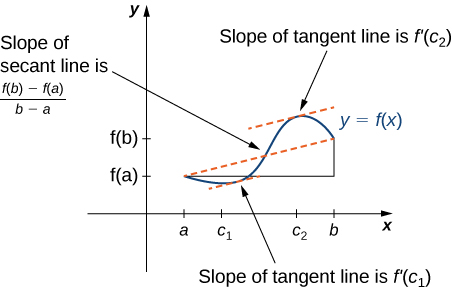
Rolle’s theorem is a special case of the Mean Value Theorem. In Rolle’s theorem, we consider differentiable functions [latex]f[/latex]defined on a closed interval [latex][a,b][/latex] with [latex]f(a)=f(b)[/latex]. The Mean Value Theorem generalizes Rolle’s theorem by considering functions that do not necessarily have equal value at the endpoints. Consequently, we can view the Mean Value Theorem as a slanted version of Rolle’s theorem (Figure 5).

A vaguely sinusoidal function y = f(x) is drawn. On the x-axis, a, c1, c2, and b are marked. On the y-axis, f(a) and f(b) are marked. The function f(x) starts at (a, f(a)), decreases to c1, increases to c2, and then decreases to (b, f(b)). A secant line is drawn between (a, f(a)) and (b, f(b)), and it is noted that this line has slope (f(b) – f(a))/(b − a). The tangent lines at c1 and c2 are drawn, and these lines are parallel to the secant line. It is noted that the slopes of these tangent lines are f’(c1) and f’(c2), respectively. — Figure 5. The Mean Value Theorem says that for a function that meets its conditions, at some point the tangent line has the same slope as the secant line between the ends. For this function, there are two values [latex]c_1[/latex] and [latex]c_2[/latex] such that the tangent line to [latex]f[/latex] at [latex]c_1[/latex] and [latex]c_2[/latex] has the same slope as the secant line.

The Mean Value Theorem states that if [latex]f[/latex] is continuous over the closed interval [latex][a,b][/latex] and differentiable over the open interval [latex](a,b)[/latex], then there exists a point [latex]c \in (a,b)[/latex] such that the tangent line to the graph of [latex]f[/latex] at [latex]c[/latex] is parallel to the secant line connecting [latex](a,f(a))[/latex] and [latex](b,f(b))[/latex].

Mean Value Theorem

Let [latex]f[/latex] be continuous over the closed interval [latex][a,b][/latex] and differentiable over the open interval [latex](a,b)[/latex]. Then, there exists at least one point [latex]c \in (a,b)[/latex] such that

[latex]f^{\prime}(c)=\dfrac{f(b)-f(a)}{b-a}[/latex]

Proof

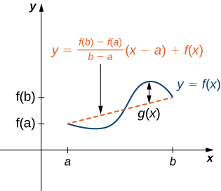
The proof follows from Rolle’s theorem by introducing an appropriate function that satisfies the criteria of Rolle’s theorem. Consider the line connecting [latex](a,f(a))[/latex] and [latex](b,f(b))[/latex]. Since the slope of that line is

[latex]\dfrac{f(b)-f(a)}{b-a}[/latex]

and the line passes through the point [latex](a,f(a))[/latex], the equation of that line can be written as

[latex]y=\dfrac{f(b)-f(a)}{b-a}(x-a)+f(a)[/latex]

Let [latex]g(x)[/latex] denote the vertical difference between the point [latex](x,f(x))[/latex] and the point [latex](x,y)[/latex] on that line. Therefore,

[latex]g(x)=f(x)-\left[\dfrac{f(b)-f(a)}{b-a}(x-a)+f(a)\right][/latex]

A vaguely sinusoidal function y = f(x) is drawn. On the x-axis, a and b are marked. On the y-axis, f(a) and f(b) are marked. The function f(x) starts at (a, f(a)), decreases, then increases, and then decreases to (b, f(b)). A secant line is drawn between (a, f(a)) and (b, f(b)), and it is noted that this line has equation y = ((f(b) – f(a))/(b − a)) (x − a) + f(x). A line is drawn between the maximum of f(x) and the secant line and it is marked g(x). — Figure 6. The value [latex]g(x)[/latex] is the vertical difference between the point [latex](x,f(x))[/latex] and the point [latex](x,y)[/latex] on the secant line connecting [latex](a,f(a))[/latex] and [latex](b,f(b)).[/latex]

Since the graph of [latex]f[/latex] intersects the secant line when [latex]x=a[/latex] and [latex]x=b[/latex], we see that [latex]g(a)=0=g(b)[/latex]. Since [latex]f[/latex] is a differentiable function over [latex](a,b)[/latex], [latex]g[/latex] is also a differentiable function over [latex](a,b)[/latex]. Furthermore, since [latex]f[/latex] is continuous over [latex][a,b][/latex], [latex]g[/latex] is also continuous over [latex][a,b][/latex]. Therefore, [latex]g[/latex] satisfies the criteria of Rolle’s theorem. Consequently, there exists a point [latex]c \in (a,b)[/latex] such that [latex]g^{\prime}(c)=0[/latex]. Since

[latex]g^{\prime}(x)=f^{\prime}(x)-\dfrac{f(b)-f(a)}{b-a}[/latex],

we see that

[latex]g^{\prime}(c)=f^{\prime}(c)-\dfrac{f(b)-f(a)}{b-a}[/latex]

Since [latex]g^{\prime}(c)=0[/latex], we conclude that

[latex]f^{\prime}(c)=\dfrac{f(b)-f(a)}{b-a}[/latex]

[latex]_\blacksquare[/latex]

In the next example, we show how the Mean Value Theorem can be applied to the function [latex]f(x)=\sqrt{x}[/latex] over the interval [latex][0,9][/latex]. The method is the same for other functions, although sometimes with more interesting consequences.

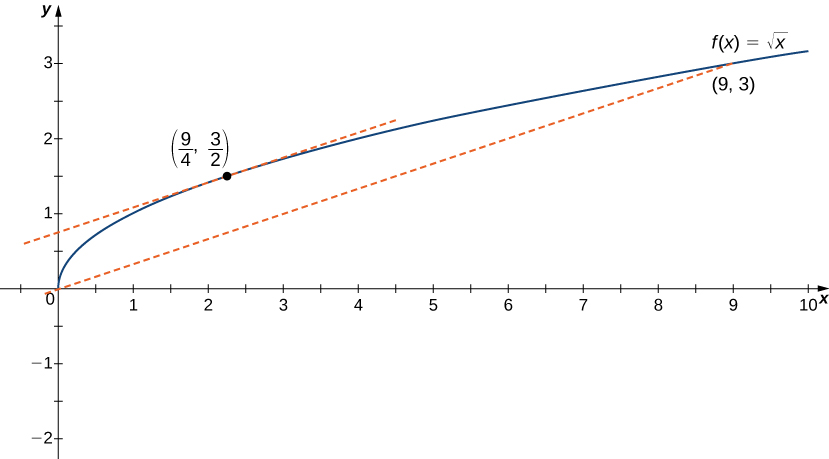
For [latex]f(x)=\sqrt{x}[/latex] over the interval [latex][0,9][/latex], show that [latex]f[/latex] satisfies the hypothesis of the Mean Value Theorem, and therefore there exists at least one value [latex]c \in (0,9)[/latex] such that [latex]f^{\prime}(c)[/latex] is equal to the slope of the line connecting [latex](0,f(0))[/latex] and [latex](9,f(9))[/latex]. Find these values [latex]c[/latex] guaranteed by the Mean Value Theorem.

One application that helps illustrate the Mean Value Theorem involves velocity.

Suppose we drive a car for [latex]1[/latex] hr down a straight road with an average velocity of [latex]45[/latex] mph.

Let [latex]s(t)[/latex] and [latex]v(t)[/latex] denote the position and velocity of the car, respectively, for [latex]0 \le t \le 1[/latex] hr. Assuming that the position function [latex]s(t)[/latex] is differentiable, we can apply the Mean Value Theorem to conclude that, at some time [latex]c \in (0,1)[/latex], the speed of the car was exactly

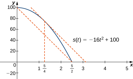
[latex]v(c)=s^{\prime}(c)=\dfrac{s(1)-s(0)}{1-0}=45[/latex] mph

If a rock is dropped from a height of [latex]100[/latex] ft, its position [latex]t[/latex] seconds after it is dropped until it hits the ground is given by the function [latex]s(t)=-16t^2+100[/latex].

Determine how long it takes before the rock hits the ground.
Find the average velocity [latex]v_{\text{avg}}[/latex] of the rock for when the rock is released and the rock hits the ground.
Find the time [latex]t[/latex] guaranteed by the Mean Value Theorem when the instantaneous velocity of the rock is [latex]v_{\text{avg}}[/latex].

When the rock hits the ground, its position is [latex]s(t)=0[/latex]. Solving the equation [latex]-16t^2+100=0[/latex] for [latex]t[/latex], we find that [latex]t=\pm \frac{5}{2}[/latex] sec. Since we are only considering [latex]t \ge 0[/latex], the ball will hit the ground [latex]\frac{5}{2}[/latex] sec after it is dropped.
The average velocity is given by:
[latex]v_{\text{avg}}=\frac{s(5/2)-s(0)}{5/2-0}=\frac{1-100}{5/2}=-40[/latex] ft/sec
The instantaneous velocity is given by the derivative of the position function. Therefore, we need to find a time [latex]t[/latex] such that [latex]v(t)=s^{\prime}(t)=v_{\text{avg}}=-40[/latex] ft/sec. Since [latex]s(t)[/latex] is continuous over the interval [latex][0,5/2][/latex] and differentiable over the interval [latex](0,5/2)[/latex], by the Mean Value Theorem, there is guaranteed to be a point [latex]c \in (0,5/2)[/latex] such that
[latex]s^{\prime}(c)=\frac{s(5/2)-s(0)}{5/2-0}=-40[/latex]

Taking the derivative of the position function [latex]s(t)[/latex], we find that [latex]s^{\prime}(t)=-32t[/latex]. Therefore, the equation reduces to [latex]s^{\prime}(c)=-32c=-40[/latex]. Solving this equation for [latex]c[/latex], we have [latex]c=\frac{5}{4}[/latex]. Therefore, [latex]\frac{5}{4}[/latex] sec after the rock is dropped, the instantaneous velocity equals the average velocity of the rock during its free fall: [latex]-40[/latex] ft/sec.

Figure 8. At time [latex]t=\frac{5}{4}[/latex] sec, the velocity of the rock is equal to its average velocity from the time it is dropped until it hits the ground.

Watch the following video to see the worked solution to this example.

For closed captioning, open the video on its original page by clicking the Youtube logo in the lower right-hand corner of the video display. In YouTube, the video will begin at the same starting point as this clip, but will continue playing until the very end.

You can view the transcript for this segmented clip of “4.4 Mean Value Theorem” here (opens in new window).

Watch the following video to see the worked solution to the two previous examples.