Graphing a Derivative
Given the equation of a function or its derivative, we can graph it to understand the relationship between the two. The derivative [latex]f^{\prime}(x)[/latex] gives the rate of change of a function [latex]f(x)[/latex] or the slope of the tangent line to [latex]f(x)[/latex]. To understand this relationship better, it is helpful to recall the characteristics of lines with certain slopes.
- Positive Slope: A line has a positive slope if it is increasing from left to right.
- Negative Slope: A line has a negative slope if it is decreasing from left to right.
- Zero Slope: A horizontal line has a slope of [latex]0[/latex].
- Undefined Slope: A vertical line has an undefined slope.
In the first example on the previous page, we found that for [latex]f(x)=\sqrt{x}, \, f^{\prime}(x)=\frac{1}{2}\sqrt{x}[/latex]. If we graph these functions on the same axes, as in Figure 2, we can use the graphs to understand the relationship between these two functions.
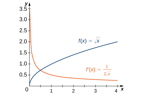
Looking at the graphs, notice that [latex]f(x)[/latex] is increasing over its entire domain, meaning the slopes of its tangent lines at all points are positive. Consequently, [latex]f^{\prime}(x)>0[/latex] for all values of [latex]x[/latex] in its domain. As [latex]x[/latex] increases, the slopes of the tangent lines to [latex]f(x)[/latex] decrease, leading to a corresponding decrease in [latex]f^{\prime}(x)[/latex]. Additionally, [latex]f(0)[/latex] is undefined and that [latex]\underset{x\to 0^+}{\lim}f^{\prime}(x)=+\infty[/latex], corresponding to a vertical tangent to [latex]f(x)[/latex] at [latex]0[/latex].
In the second example, we found that for [latex]f(x)=x^2-2x, \, f^{\prime}(x)=2x-2[/latex]. The graphs of these functions are shown in Figure 3.
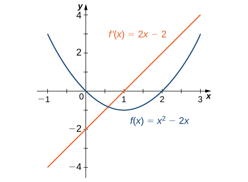
Observe that [latex]f(x)[/latex] is decreasing for [latex]x<1[/latex]. For these values of [latex]x, \, f^{\prime}(x)<0[/latex]. For [latex]x>1, \, f(x)[/latex] is increasing and [latex]f^{\prime}(x)>0[/latex]. Also, [latex]f(x)[/latex] has a horizontal tangent at [latex]x=1[/latex] and [latex]f^{\prime}(1)=0[/latex].
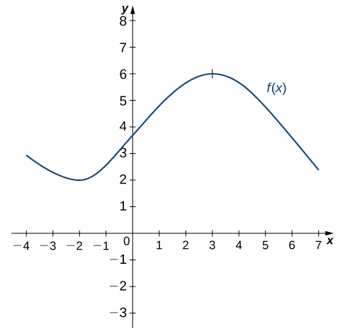
Use the following graph of [latex]f(x)[/latex] to sketch a graph of [latex]f^{\prime}(x)[/latex].