- Explain the difference between exponential growth and decay
Identify Exponential Growth and Decay
In real-world applications, we need to model the behavior of a function. In mathematical modeling, we choose a familiar general function with properties that suggest that it will model the real-world phenomenon we wish to analyze. In the case of rapid growth (or decay), we may choose to model the given scenario using the following function:
[latex]y={A}_{0}{b}^{x}[/latex]
where [latex]{A}_{0}[/latex] is equal to the value at [latex]x=0[/latex], [latex]b[/latex] is the base, and [latex]x[/latex] is the exponent. Note that the variable is in the exponent which makes the function exponential.
exponential function
For any real number [latex]x[/latex], an exponential function is a function with the form
where
- [latex]a[/latex] is a non-zero real number called the initial value and
- [latex]b[/latex] is any positive real number such that [latex]b≠1[/latex].
- The domain is [latex]\left(-\infty , \infty \right)[/latex], or all real numbers
- The range is all positive real numbers if [latex]a > 0[/latex]
- The range is all negative real numbers if [latex]a < 0[/latex]
- The y-intercept is [latex]\left(0,{A}_{0}\right)[/latex], and the horizontal asymptote is [latex]y=0[/latex]
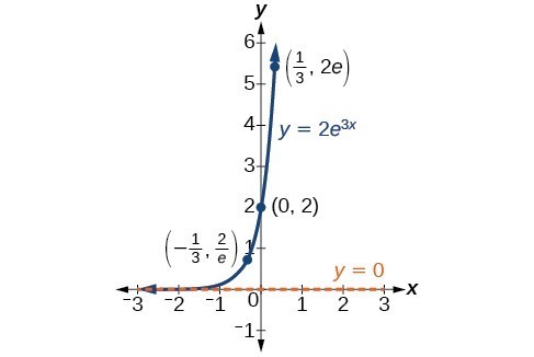
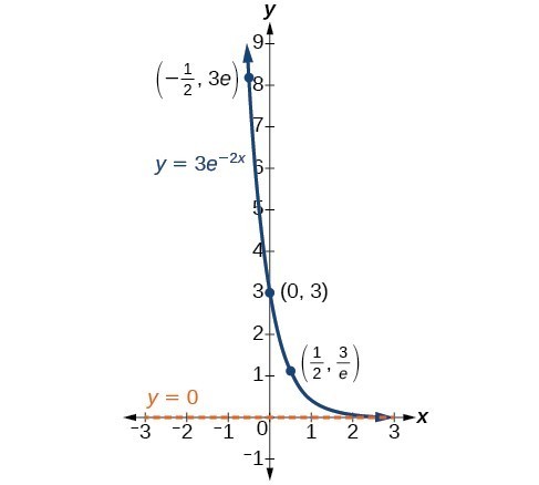
An exponential function models exponential growth when [latex]b > 1[/latex] and exponential decay when [latex]b < 1[/latex].
When [latex]b>1[/latex], the exponential function represents exponential growth. Common applications of exponential growth include doubling time, the time it takes for a quantity to double. Such phenomena as wildlife populations, financial investments, biological samples, and natural resources may exhibit growth based on a doubling time.
When [latex]b<1[/latex], the exponential function represents exponential decay. One common application of exponential decay includes calculating half-life, or the time it takes for a substance to exponentially decay to half of its original quantity. We use half-life in applications involving radioactive isotopes.
Exponential growth and decay graphs have a distinctive shape, as we can see in the graphs below. It is important to remember that, although parts of each of the two graphs seem to lie on the [latex]x[/latex]-axis, they are really a tiny distance above the [latex]x[/latex]-axis.