Maxima and Minima: Learn It 2

Lumen Learning

Maxima and Minima: Learn It 2

Extrema and Critical Points

Local Extrema and Critical Points

Consider the function [latex]f[/latex] shown in below.

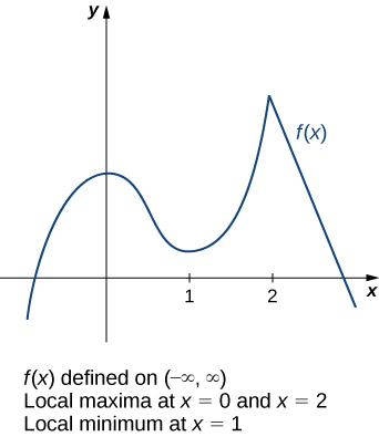
The function f(x) is shown, which curves upward from quadrant III, slows down in quadrant II, achieves a local maximum on the y-axis, decreases to achieve a local minimum in quadrant I at x = 1, increases to a local maximum at x = 2 that is greater than the other local maximum, and then decreases rapidly through quadrant IV. — Figure 3. This function [latex]f[/latex] has two local maxima and one local minimum. The local maximum at [latex]x=2[/latex] is also the absolute maximum.

The graph can be described as two mountains with a valley in the middle. The absolute maximum value of the function occurs at the higher peak, at [latex]x=2[/latex].

However, [latex]x=0[/latex] is also a point of interest. Although [latex]f(0)[/latex] is not the largest value of [latex]f[/latex], the value [latex]f(0)[/latex] is larger than [latex]f(x)[/latex] for all [latex]x[/latex] near [latex]0[/latex]. We say [latex]f[/latex] has a local maximum at [latex]x=0[/latex].

Similarly, the function [latex]f[/latex] does not have an absolute minimum, but it does have a local minimum at [latex]x=1[/latex] because [latex]f(1)[/latex] is less than [latex]f(x)[/latex] for [latex]x[/latex] near [latex]1[/latex].

local extremum

A function [latex]f[/latex] has a local maximum at [latex]c[/latex] if there exists an open interval [latex]I[/latex] containing [latex]c[/latex] such that [latex]I[/latex] is contained in the domain of [latex]f[/latex] and [latex]f(c)\ge f(x)[/latex] for all [latex]x\in I[/latex].

A function [latex]f[/latex] has a local minimum at [latex]c[/latex] if there exists an open interval [latex]I[/latex] containing [latex]c[/latex] such that [latex]I[/latex] is contained in the domain of [latex]f[/latex] and [latex]f(c)\le f(x)[/latex] for all [latex]x\in I[/latex].

A function [latex]f[/latex] has a local extremum at [latex]c[/latex] if [latex]f[/latex] has a local maximum at [latex]c[/latex] or [latex]f[/latex] has a local minimum at [latex]c[/latex].

Note that if [latex]f[/latex] has an absolute extremum at [latex]c[/latex] and [latex]f[/latex] is defined over an interval containing [latex]c[/latex], then [latex]f(c)[/latex] is also considered a local extremum. If an absolute extremum for a function [latex]f[/latex] occurs at an endpoint, we do not consider that to be a local extremum, but instead refer to that as an endpoint extremum.

Given the graph of a function [latex]f[/latex], it is sometimes easy to see where a local maximum or local minimum occurs. However, it is not always easy to see, since the interesting features on the graph of a function may not be visible because they occur at a very small scale. Also, we may not have a graph of the function.

In these cases, how can we use a formula for a function to determine where these extrema occur?

To answer this question, let’s look at Figure 3 again.

The local extrema occur at [latex]x=0[/latex], [latex]x=1[/latex], and [latex]x=2[/latex]. Notice that at [latex]x=0[/latex] and [latex]x=1[/latex], the derivative [latex]f^{\prime}(x)=0[/latex]. At [latex]x=2[/latex], the derivative [latex]f^{\prime}(x)[/latex] does not exist, since the function [latex]f[/latex] has a corner there.

In fact, if [latex]f[/latex] has a local extremum at a point [latex]x=c[/latex], the derivative [latex]f^{\prime}(c)[/latex] must satisfy one of the following conditions: either [latex]f^{\prime}(c)=0[/latex] or [latex]f^{\prime}(c)[/latex] is undefined.

Such a value [latex]c[/latex] is known as a critical point and it is important in finding extreme values for functions.

critical point

Let [latex]c[/latex] be an interior point in the domain of [latex]f[/latex]. We say that [latex]c[/latex] is a critical point of [latex]f[/latex] if [latex]f^{\prime}(c)=0[/latex] or [latex]f^{\prime}(c)[/latex] is undefined.

As mentioned earlier, if [latex]f[/latex] has a local extremum at a point [latex]x=c[/latex], then [latex]c[/latex] must be a critical point of [latex]f[/latex]. This fact is known as Fermat’s theorem.

Fermat’s theorem

If [latex]f[/latex] has a local extremum at [latex]c[/latex] and [latex]f[/latex] is differentiable at [latex]c[/latex], then [latex]f^{\prime}(c)=0[/latex].

Proof

Suppose [latex]f[/latex] has a local extremum at [latex]c[/latex] and [latex]f[/latex] is differentiable at [latex]c[/latex]. We need to show that [latex]f^{\prime}(c)=0[/latex]. To do this, we will show that [latex]f^{\prime}(c)\ge 0[/latex] and [latex]f^{\prime}(c)\le 0[/latex], and therefore [latex]f^{\prime}(c)=0[/latex]. Since [latex]f[/latex] has a local extremum at [latex]c[/latex], [latex]f[/latex] has a local maximum or local minimum at [latex]c[/latex]. Suppose [latex]f[/latex] has a local maximum at [latex]c[/latex]. The case in which [latex]f[/latex] has a local minimum at [latex]c[/latex] can be handled similarly. There then exists an open interval [latex]I[/latex] such that [latex]f(c)\ge f(x)[/latex] for all [latex]x\in I[/latex]. Since [latex]f[/latex] is differentiable at [latex]c[/latex], from the definition of the derivative, we know that

[latex]f^{\prime}(c)=\underset{x\to c}{\lim}\dfrac{f(x)-f(c)}{x-c}[/latex]

Since this limit exists, both one-sided limits also exist and equal [latex]f^{\prime}(c)[/latex]. Therefore,

[latex]f^{\prime}(c)=\underset{x\to c^+}{\lim}\dfrac{f(x)-f(c)}{x-c}[/latex],

and

[latex]f^{\prime}(c)=\underset{x\to c^-}{\lim}\dfrac{f(x)-f(c)}{x-c}[/latex]

Since [latex]f(c)[/latex] is a local maximum, we see that [latex]f(x)-f(c)\le 0[/latex] for [latex]x[/latex] near [latex]c[/latex]. Therefore, for [latex]x[/latex] near [latex]c[/latex], but [latex]x>c[/latex], we have [latex]\frac{f(x)-f(c)}{x-c}\le 0[/latex]. From the equations above we conclude that [latex]f^{\prime}(c)\le 0[/latex]. Similarly, it can be shown that [latex]f^{\prime}(c)\ge 0[/latex]. Therefore, [latex]f^{\prime}(c)=0[/latex].

[latex]_\blacksquare[/latex]

From Fermat’s theorem, we conclude that if [latex]f[/latex] has a local extremum at [latex]c[/latex], then either [latex]f^{\prime}(c)=0[/latex] or [latex]f^{\prime}(c)[/latex] is undefined. In other words, local extrema can only occur at critical points.

Note this theorem does not claim that a function [latex]f[/latex] must have a local extremum at a critical point. Rather, it states that critical points are candidates for local extrema.

Consider the function [latex]f(x)=x^3[/latex]. We have [latex]f^{\prime}(x)=3x^2=0[/latex] when [latex]x=0[/latex]. Therefore, [latex]x=0[/latex] is a critical point. However, [latex]f(x)=x^3[/latex] is increasing over [latex](−\infty ,\infty )[/latex], and thus [latex]f[/latex] does not have a local extremum at [latex]x=0[/latex].

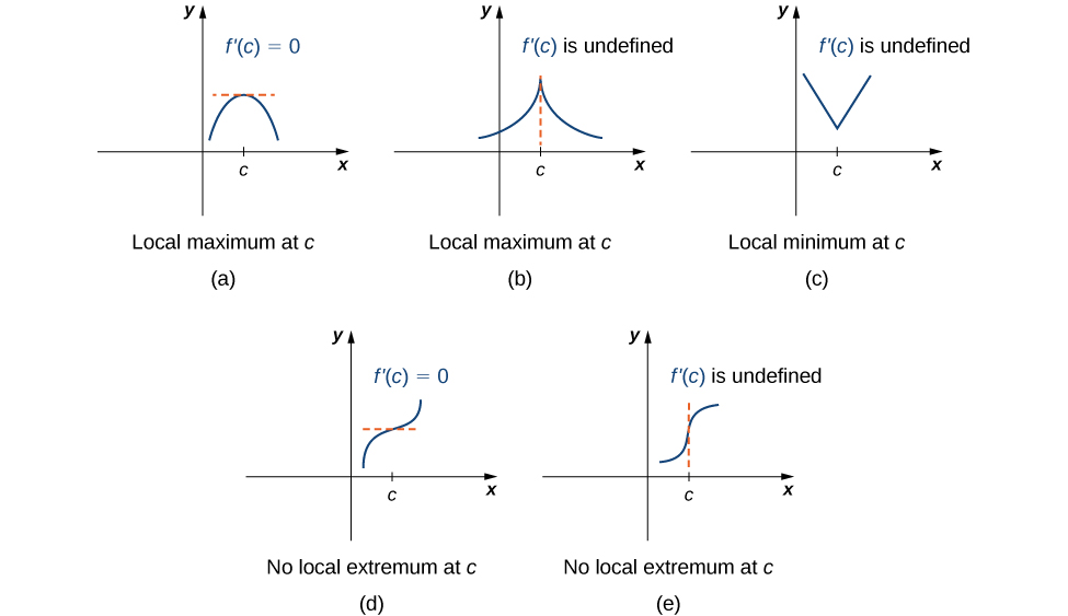
In Figure 4, we see several different possibilities for critical points. In some of these cases, the functions have local extrema at critical points, whereas in other cases the functions do not. Note that these graphs do not show all possibilities for the behavior of a function at a critical point.

This figure has five parts a, b, c, d, and e. In figure a, a parabola is shown facing down in quadrant I; there is a horizontal tangent line at the local maximum marked f’(c) = 0. In figure b, there is a function drawn with an asymptote at c, meaning that the function increases toward infinity on both sides of c; it is noted that f’(c) is undefined. In figure c, a version of the absolute value graph is shown that has been shifted so that its minimum is in quadrant I with x = c. It is noted that f’(c) is undefined. In figure d, a version of the function f(x) = x3 is shown that has been shifted so that its inflection point is in quadrant I with x = c. Its inflection point at (c, f(c)) has a horizontal line through it, and it is noted that f’(c) = 0. In figure e, a version of the function f(x) = x1/3 is shown that has been shifted so that its inflection point is in quadrant I with x = c. Its inflection point at (c, f(c)) has a vertical line through it, and it is noted that f’(c) is undefined. — Figure 4. (a–e) A function [latex]f[/latex] has a critical point at [latex]c[/latex] if [latex]f^{\prime}(c)=0[/latex] or [latex]f^{\prime}(c)[/latex] is undefined. A function may or may not have a local extremum at a critical point.

Later in this module we look at analytical methods for determining whether a function actually has a local extremum at a critical point. For now, let’s turn our attention to finding critical points. We will use graphical observations to determine whether a critical point is associated with a local extremum.

For each of the following functions, find all critical points. Use a graphing utility to determine whether the function has a local extremum at each of the critical points.

[latex]f(x)=\frac{1}{3}x^3-\frac{5}{2}x^2+4x[/latex]
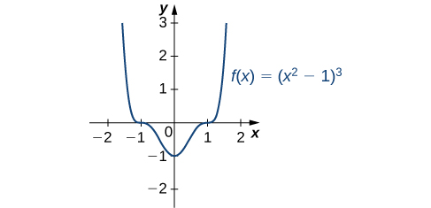
[latex]f(x)=(x^2-1)^3[/latex]
[latex]f(x)=\dfrac{4x}{1+x^2}[/latex]

The derivative [latex]f^{\prime}(x)=x^2-5x+4[/latex] is defined for all real numbers [latex]x[/latex]. Therefore, we only need to find the values for [latex]x[/latex] where [latex]f^{\prime}(x)=0[/latex]. Since [latex]f^{\prime}(x)=x^2-5x+4=(x-4)(x-1)[/latex], the critical points are [latex]x=1[/latex] and [latex]x=4[/latex]. From the graph of [latex]f[/latex] in Figure 5, we see that [latex]f[/latex] has a local maximum at [latex]x=1[/latex] and a local minimum at [latex]x=4[/latex].

Figure 5. This function has a local maximum and a local minimum.
Using the chain rule, we see the derivative is
[latex]f^{\prime}(x)=3(x^2-1)^2(2x)=6x(x^2-1)^2[/latex]

Therefore, [latex]f[/latex] has critical points when [latex]x=0[/latex] and when [latex]x^2-1=0[/latex]. We conclude that the critical points are [latex]x=0,\pm 1[/latex]. From the graph of [latex]f[/latex] in Figure 6, we see that [latex]f[/latex] has a local (and absolute) minimum at [latex]x=0[/latex], but does not have a local extremum at [latex]x=1[/latex] or [latex]x=-1[/latex].

Figure 6. This function has three critical points: [latex]x=0[/latex], [latex]x=1[/latex], and [latex]x=-1[/latex]. The function has a local (and absolute) minimum at [latex]x=0[/latex], but does not have extrema at the other two critical points.
By the chain rule, we see that the derivative is
[latex]f^{\prime}(x)=\dfrac{(1+x^2 \cdot 4)-4x(2x)}{(1+x^2)^2}=\dfrac{4-4x^2}{(1+x^2)^2}[/latex]

The derivative is defined everywhere. Therefore, we only need to find values for [latex]x[/latex] where [latex]f^{\prime}(x)=0[/latex]. Solving [latex]f^{\prime}(x)=0[/latex], we see that [latex]4-4x^2=0[/latex], which implies [latex]x=\pm 1[/latex]. Therefore, the critical points are [latex]x=\pm 1[/latex]. From the graph of [latex]f[/latex] in Figure 7, we see that [latex]f[/latex] has an absolute maximum at [latex]x=1[/latex] and an absolute minimum at [latex]x=-1[/latex]. Hence, [latex]f[/latex] has a local maximum at [latex]x=1[/latex] and a local minimum at [latex]x=-1[/latex]. (Note that if [latex]f[/latex] has an absolute extremum over an interval [latex]I[/latex] at a point [latex]c[/latex] that is not an endpoint of [latex]I[/latex], then [latex]f[/latex] has a local extremum at [latex]c[/latex].)

Figure 7. This function has an absolute maximum and an absolute minimum.

Watch the following video to see the worked solution to this example.

For closed captioning, open the video on its original page by clicking the Youtube logo in the lower right-hand corner of the video display. In YouTube, the video will begin at the same starting point as this clip, but will continue playing until the very end.

You can view the transcript for this segmented clip of “4.3 Maxima and Minima” here (opens in new window).