- Define and Identify the highest and lowest points of a function on a graph, both overall and within specific sections
- Locate points on a function within a specific range where the slope is zero or undefined (critical points)
- Explain how to use critical points to find the highest or lowest values of a function within a limited range
Extrema and Critical Points
Given a particular function, we are often interested in determining the largest and smallest values of the function. This information is important in creating accurate graphs. Finding the maximum and minimum values of a function also has practical significance because we can use this method to solve optimization problems, such as maximizing profit, minimizing the amount of material used in manufacturing an aluminum can, or finding the maximum height a rocket can reach. In this section, we look at how to use derivatives to find the largest and smallest values for a function.
Absolute Extrema
Consider the function [latex]f(x)=x^2+1[/latex] over the interval [latex](−\infty ,\infty )[/latex]. As [latex]x\to \pm \infty[/latex], [latex]f(x)\to \infty[/latex]. Therefore, the function does not have a largest value. However, since [latex]x^2+1\ge 1[/latex] for all real numbers [latex]x[/latex] and [latex]x^2+1=1[/latex] when [latex]x=0[/latex], the function has a smallest value, [latex]1[/latex], when [latex]x=0[/latex].
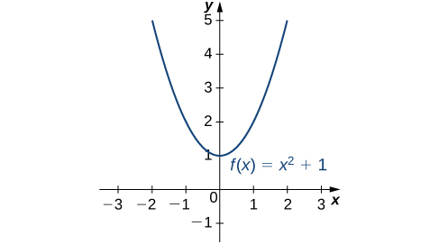
We say that [latex]1[/latex] is the absolute minimum of [latex]f(x)=x^2+1[/latex] and it occurs at [latex]x=0[/latex]. We say that [latex]f(x)=x^2+1[/latex] does not have an absolute maximum.
absolute maximum and extremum
Let [latex]f[/latex] be a function defined over an interval [latex]I[/latex] and let [latex]c\in I[/latex].
We say [latex]f[/latex] has an absolute maximum on [latex]I[/latex] at [latex]c[/latex] if [latex]f(c)\ge f(x)[/latex] for all [latex]x\in I[/latex].
We say [latex]f[/latex] has an absolute minimum on [latex]I[/latex] at [latex]c[/latex] if [latex]f(c)\le f(x)[/latex] for all [latex]x\in I[/latex].
If [latex]f[/latex] has an absolute maximum on [latex]I[/latex] at [latex]c[/latex] or an absolute minimum on [latex]I[/latex] at [latex]c[/latex], we say [latex]f[/latex] has an absolute extremum on [latex]I[/latex] at [latex]c[/latex].
Before proceeding, let’s note two important issues regarding this definition.
First, the term absolute here does not refer to absolute value. An absolute extremum may be positive, negative, or zero.
Second, if a function [latex]f[/latex] has an absolute extremum over an interval [latex]I[/latex] at [latex]c[/latex], the absolute extremum is [latex]f(c)[/latex]. The real number [latex]c[/latex] is a point in the domain at which the absolute extremum occurs.
Consider the function [latex]f(x)=\frac{1}{(x^2+1)}[/latex] over the interval [latex](−\infty ,\infty )[/latex]. Since
for all real numbers [latex]x[/latex], we say [latex]f[/latex] has an absolute maximum over [latex](−\infty ,\infty )[/latex] at [latex]x=0[/latex]. The absolute maximum is [latex]f(0)=1[/latex]. It occurs at [latex]x=0[/latex], as shown in Figure 2b.
So remember: the maximum/minimum = [latex]y[/latex]; the location of the maximum/minimum = [latex]x[/latex].
A function may have both an absolute maximum and an absolute minimum, just one extremum, or neither. Figure 2 shows several functions and some of the different possibilities regarding absolute extrema.
![This figure has six parts a, b, c, d, e, and f. In figure a, the line f(x) = x3 is shown, and it is noted that it has no absolute minimum and no absolute maximum. In figure b, the line f(x) = 1/(x2 + 1) is shown, which is near 0 for most of its length and rises to a bump at (0, 1); it has no absolute minimum, but does have an absolute maximum of 1 at x = 0. In figure c, the line f(x) = cos x is shown, which has absolute minimums of −1 at ±π, ±3π, … and absolute maximums of 1 at 0, ±2π, ±4π, …. In figure d, the piecewise function f(x) = 2 – x2 for 0 ≤ x < 2 and x – 3 for 2 ≤ x ≤ 4 is shown, with absolute maximum of 2 at x = 0 and no absolute minimum. In figure e, the function f(x) = (x – 2)2 is shown on [1, 4], which has absolute maximum of 4 at x = 4 and absolute minimum of 0 at x = 2. In figure f, the function f(x) = x/(2 − x) is shown on [0, 2), with absolute minimum of 0 at x = 0 and no absolute maximum.](https://s3-us-west-2.amazonaws.com/courses-images/wp-content/uploads/sites/2332/2018/01/11210805/CNX_Calc_Figure_04_03_010.jpg)
However, the following theorem, called the extreme value theorem, guarantees that a continuous function [latex]f[/latex] over a closed, bounded interval [latex][a,b][/latex] has both an absolute maximum and an absolute minimum.
extreme value theorem
If [latex]f[/latex] is a continuous function over the closed, bounded interval [latex][a,b][/latex], then there is a point in [latex][a,b][/latex] at which [latex]f[/latex] has an absolute maximum over [latex][a,b][/latex] and there is a point in [latex][a,b][/latex] at which [latex]f[/latex] has an absolute minimum over [latex][a,b][/latex].
The proof of the extreme value theorem is beyond the scope of this text. Typically, it is proved in a course on real analysis.
There are a couple of key points to note about the statement of this theorem. For the extreme value theorem to apply, the function must be continuous over a closed, bounded interval. If the interval [latex]I[/latex] is open or the function has even one point of discontinuity, the function may not have an absolute maximum or absolute minimum over [latex]I[/latex].
Consider the functions shown in Figure 2(d), (e), and (f).
All three of these functions are defined over bounded intervals. However, the function in graph (e) is the only one that has both an absolute maximum and an absolute minimum over its domain.
The extreme value theorem cannot be applied to the functions in graphs (d) and (f) because neither of these functions is continuous over a closed, bounded interval.
Although the function in graph (d) is defined over the closed interval [latex][0,4][/latex], the function is discontinuous at [latex]x=2[/latex]. The function has an absolute maximum over [latex][0,4][/latex] but does not have an absolute minimum.
The function in graph (f) is continuous over the half-open interval [latex][0,2)[/latex], but is not defined at [latex]x=2[/latex], and therefore is not continuous over a closed, bounded interval. The function has an absolute minimum over [latex][0,2)[/latex], but does not have an absolute maximum over [latex][0,2)[/latex].
These two graphs illustrate why a function over a bounded interval may fail to have an absolute maximum and/or absolute minimum.
Before looking at how to find absolute extrema, let’s examine the related concept of local extrema. This idea is useful in determining where absolute extrema occur.