Linear Approximation of a Function at a Point

We have just seen how derivatives allow us to compare related quantities that are changing over time. In this section, we examine another application of derivatives: the ability to approximate functions locally by linear functions. Linear functions are the easiest functions with which to work, so they provide a useful tool for approximating function values.

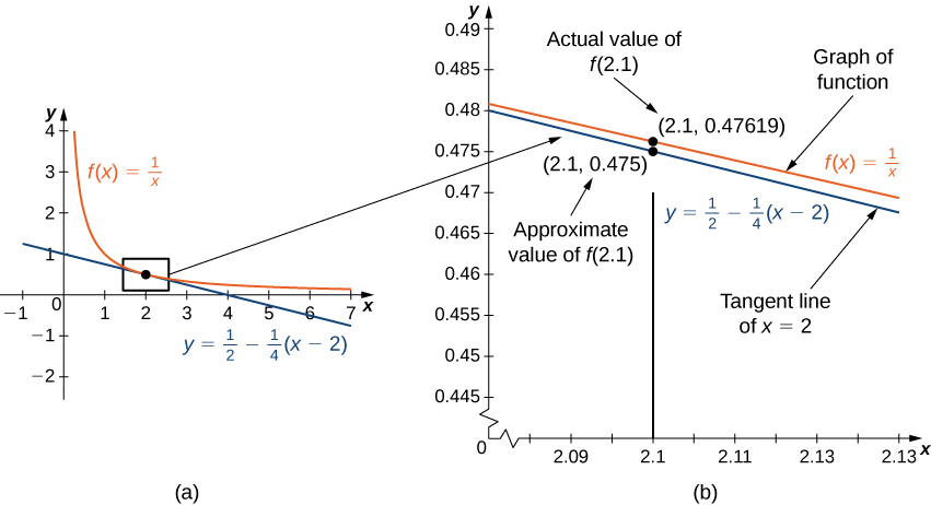
Consider the function [latex]f(x)=\frac{1}{x}[/latex] at [latex]a=2[/latex]. Since [latex]f[/latex] is differentiable at [latex]x=2[/latex] and [latex]f^{\prime}(x)=-\frac{1}{x^2}[/latex], we see that [latex]f^{\prime}(2)=-\frac{1}{4}[/latex].

Therefore, the tangent line to the graph of [latex]f[/latex] at [latex]a=2[/latex] is given by the equation

Figure 1a shows a graph of [latex]f(x)=\frac{1}{x}[/latex] along with the tangent line to [latex]f[/latex] at [latex]x=2[/latex]. Note that for [latex]x[/latex] near [latex]2[/latex], the graph of the tangent line is close to the graph of [latex]f[/latex]. As a result, we can use the equation of the tangent line to approximate [latex]f(x)[/latex] for [latex]x[/latex] near [latex]2[/latex].

If [latex]x=2.1[/latex], the [latex]y[/latex] value of the corresponding point on the tangent line is

The actual value of [latex]f(2.1)[/latex] is given by

Therefore, the tangent line gives us a fairly good approximation of [latex]f(2.1)[/latex] (Figure 1b).

However, note that for values of [latex]x[/latex] far from [latex]2[/latex], the equation of the tangent line does not give us a good approximation. If [latex]x=10[/latex], the [latex]y[/latex]-value of the corresponding point on the tangent line is

whereas the value of the function at [latex]x=10[/latex] is [latex]f(10)=0.1[/latex].

In general, for a differentiable function [latex]f[/latex], the equation of the tangent line to [latex]f[/latex] at [latex]x=a[/latex] can be used to approximate [latex]f(x)[/latex] for [latex]x[/latex] near [latex]a[/latex]. Therefore, we can write

We call the linear function

the linear approximation, or tangent line approximation, of [latex]f[/latex] at [latex]x=a[/latex]. This function [latex]L[/latex] is also known as the linearization of [latex]f[/latex] at [latex]x=a[/latex].

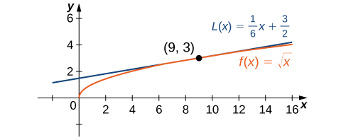
Find the linear approximation of [latex]f(x)=\sqrt{x}[/latex] at [latex]x=9[/latex] and use the approximation to estimate [latex]\sqrt{9.1}[/latex].

Show Solution

Since we are looking for the linear approximation at [latex]x=9[/latex], using the tangent line approximation, we know the linear approximation is given by

[latex]L(x)=f(9)+f^{\prime}(9)(x-9)[/latex].

We need to find [latex]f(9)[/latex] and [latex]f^{\prime}(9)[/latex].

[latex]\begin{array}{lll} f(x)=\sqrt{x}& \Rightarrow & f(9)=\sqrt{9}=3 \\ f^{\prime}(x)=\frac{1}{2\sqrt{x}}& \Rightarrow & f^{\prime}(9)=\frac{1}{2\sqrt{9}}=\frac{1}{6} \end{array}[/latex]

Therefore, the linear approximation is given by Figure 2.

[latex]L(x)=3+\frac{1}{6}(x-9)[/latex]

Using the linear approximation, we can estimate [latex]\sqrt{9.1}[/latex] by writing

[latex]\sqrt{9.1}=f(9.1)\approx L(9.1)=3+\frac{1}{6}(9.1-9)\approx 3.0167[/latex].

Analysis

Using a calculator, the value of [latex]\sqrt{9.1}[/latex] to four decimal places is 3.0166. The value given by the linear approximation, 3.0167, is very close to the value obtained with a calculator, so it appears that using this linear approximation is a good way to estimate [latex]\sqrt{x}[/latex], at least for [latex]x[/latex] near 9. At the same time, it may seem odd to use a linear approximation when we can just push a few buttons on a calculator to evaluate [latex]\sqrt{9.1}[/latex]. However, how does the calculator evaluate [latex]\sqrt{9.1}[/latex]? The calculator uses an approximation! In fact, calculators and computers use approximations all the time to evaluate mathematical expressions; they just use higher-degree approximations.

Watch the following video to see the worked solution to this example.

For closed captioning, open the video on its original page by clicking the Youtube logo in the lower right-hand corner of the video display. In YouTube, the video will begin at the same starting point as this clip, but will continue playing until the very end.

You can view the transcript for this segmented clip of “4.2 Linear Approximations and Differentials” here (opens in new window).

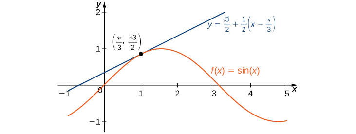
Find the linear approximation of [latex]f(x)= \sin x[/latex] at [latex]x=\dfrac{\pi}{3}[/latex] and use it to approximate [latex]\sin (62^{\circ})[/latex].

Show Solution

First we note that since [latex]\frac{\pi}{3}[/latex] rad is equivalent to [latex]60^{\circ}[/latex], using the linear approximation at [latex]x=\pi /3[/latex] seems reasonable. The linear approximation is given by

[latex]L(x)=f(\frac{\pi}{3})+f^{\prime}(\frac{\pi}{3})(x-\frac{\pi}{3})[/latex].

We see that

[latex]\begin{array}{lll}f(x)= \sin x & \Rightarrow & f(\frac{\pi}{3})= \sin (\frac{\pi}{3})=\frac{\sqrt{3}}{2} \\ f^{\prime}(x)= \cos x & \Rightarrow & f^{\prime}(\frac{\pi}{3})= \cos (\frac{\pi}{3})=\frac{1}{2} \end{array}[/latex]

Therefore, the linear approximation of [latex]f[/latex] at [latex]x=\pi /3[/latex] is given by Figure 3.

[latex]L(x)=\frac{\sqrt{3}}{2}+\frac{1}{2}(x-\frac{\pi}{3})[/latex]

To estimate [latex]\sin (62^{\circ})[/latex] using [latex]L[/latex], we must first convert [latex]62^{\circ}[/latex] to radians. We have [latex]62^{\circ}=\frac{62\pi}{180}[/latex] radians, so the estimate for [latex]\sin (62^{\circ})[/latex] is given by

[latex]\sin (62^{\circ})=f(\frac{62\pi}{180})\approx L(\frac{62\pi }{180})=\frac{\sqrt{3}}{2}+\frac{1}{2}(\frac{62\pi }{180}-\frac{\pi }{3})=\frac{\sqrt{3}}{2}+\frac{1}{2}(\frac{2\pi }{180})=\frac{\sqrt{3}}{2}+\frac{\pi }{180}\approx 0.88348[/latex].

Watch the following video to see the worked solution to this example.

For closed captioning, open the video on its original page by clicking the Youtube logo in the lower right-hand corner of the video display. In YouTube, the video will begin at the same starting point as this clip, but will continue playing until the very end.

You can view the transcript for this segmented clip of “4.2 Linear Approximations and Differentials” here (opens in new window).

Linear approximations may be used in estimating roots and powers. In the next example, we find the linear approximation for [latex]f(x)=(1+x)^n[/latex] at [latex]x=0[/latex], which can be used to estimate roots and powers for real numbers near [latex]1[/latex]. The same idea can be extended to a function of the form [latex]f(x)=(m+x)^n[/latex] to estimate roots and powers near a different number [latex]m[/latex].

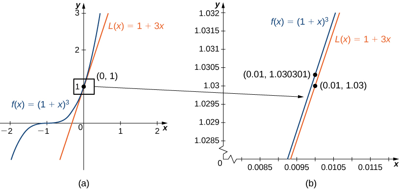
Find the linear approximation of [latex]f(x)=(1+x)^n[/latex] at [latex]x=0[/latex]. Use this approximation to estimate [latex](1.01)^3[/latex].

Show Solution

The linear approximation at [latex]x=0[/latex] is given by

[latex]L(x)=f(0)+f^{\prime}(0)(x-0)[/latex].

 

Because

[latex]\begin{array}{lll} f(x)=(1+x)^n & \Rightarrow & f(0)=1 \\ f^{\prime}(x)=n(1+x)^{n-1} & \Rightarrow & f^{\prime}(0)=n, \end{array}[/latex]

 

the linear approximation is given by Figure 4a.

[latex]L(x)=1+n(x-0)=1+nx[/latex]

 

We can approximate [latex](1.01)^3[/latex] by evaluating [latex]L(0.01)[/latex] when [latex]n=3[/latex]. We conclude that

[latex](1.01)^3=f(1.01)\approx L(1.01)=1+3(0.01)=1.03[/latex].