Limits at Infinity and Asymptotes: Learn It 3

Lumen Learning

Limits at Infinity and Asymptotes: Learn It 3

End Behavior

The behavior of a function as $x\to \pm \infty$ is called the function’s end behavior. At each of the function’s ends, the function could exhibit one of the following types of behavior:

The function $f(x)$ approaches a horizontal asymptote $y=L$ .
The function $f(x)\to \infty$ or $f(x)\to −\infty$ .
The function does not approach a finite limit, nor does it approach $\infty$ or $−\infty$ . In this case, the function may have some oscillatory behavior.

Let’s consider several classes of functions here and look at the different types of end behaviors for these functions.

End Behavior for Polynomial Functions

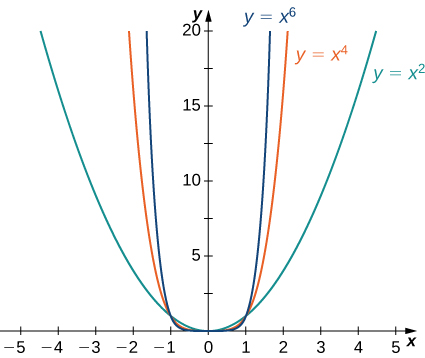
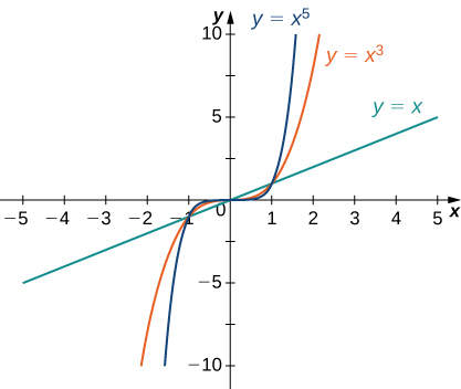
Consider the power function $f(x)=x^n$ where $n$ is a positive integer. From Figure 11 and Figure 12, we see that,

lim x \to \infty x^{n} = \infty; n = 1, 2, 3, \dots

$\underset{x\to \infty }{\lim}x^n=\infty; \, n=1,2,3, \cdots$

and,

lim x \to - \infty x^{n} = {\begin{matrix} \infty; & n = 2, 4, 6, \dots - \infty; & n = 1, 3, 5, \dots \end{matrix}

$\underset{x\to −\infty }{\lim}x^n=\begin{cases} \infty; & n=2,4,6,\cdots \\ -\infty; & n=1,3,5,\cdots \end{cases}$

The functions x2, x4, and x6 are graphed, and it is apparent that as the exponent grows the functions increase more quickly. — Figure 11. For power functions with an even power of $n$ , $\underset{x\to \infty }{\lim}x^n=\infty =\underset{x\to −\infty }{\lim}x^n$ .

The functions x, x3, and x5 are graphed, and it is apparent that as the exponent grows the functions increase more quickly. — Figure 12. For power functions with an odd power of $n$ , $\underset{x\to \infty }{\lim}x^n=\infty$ and $\underset{x\to −\infty}{\lim}x^n=−\infty$ .

Using these facts, it is not difficult to evaluate $\underset{x\to \infty }{\lim}cx^n$ and $\underset{x\to −\infty }{\lim}cx^n$ , where $c$ is any constant and $n$ is a positive integer.

evaluating limits of power functions

If $c>0$ , the graph of $y=cx^n$ is a vertical stretch or compression of $y=x^n$ , and therefore,

lim x \to \infty c x^{n} = lim x \to \infty x^{n}

$\underset{x\to \infty }{\lim}cx^n=\underset{x\to \infty }{\lim}x^n$ and

lim x \to - \infty c x^{n} = lim x \to - \infty x^{n}

$\underset{x\to −\infty }{\lim}cx^n=\underset{x\to −\infty}{\lim}x^n$ if

c > 0

$c>0$

If $c<0$ , the graph of $y=cx^n$ is a vertical stretch or compression combined with a reflection about the $x$ -axis, and therefore,

lim x \to \infty c x^{n} = - lim x \to \infty x^{n}

$\underset{x\to \infty }{\lim}cx^n=−\underset{x\to \infty }{\lim}x^n$ and

lim x \to - \infty c x^{n} = - lim x \to - \infty x^{n}

$\underset{x\to −\infty}{\lim}cx^n=−\underset{x\to −\infty }{\lim}x^n$ if

c < 0

$c<0$

If $c=0, \, y=cx^n=0$ , in which case $\underset{x\to \infty }{\lim}cx^n=0=\underset{x\to −\infty }{\lim}cx^n$ .

For each function $f$ , evaluate $\underset{x\to \infty }{\lim}f(x)$ and $\underset{x\to −\infty }{\lim}f(x)$ .

$f(x)=-5x^3$
$f(x)=2x^4$

Since the coefficient of $x^3$ is $-5$ , the graph of $f(x)=-5x^3$ involves a vertical stretch and reflection of the graph of $y=x^3$ about the $x$ -axis. Therefore, $\underset{x\to \infty }{\lim}(-5x^3)=−\infty$ and $\underset{x\to −\infty }{\lim}(-5x^3)=\infty$ .
Since the coefficient of $x^4$ is $2$ , the graph of $f(x)=2x^4$ is a vertical stretch of the graph of $y=x^4$ . Therefore, $\underset{x\to \infty }{\lim}2x^4=\infty$ and $\underset{x\to −\infty }{\lim}2x^4=\infty$ .

Watch the following video to see the worked solution to this example.

For closed captioning, open the video on its original page by clicking the Youtube logo in the lower right-hand corner of the video display. In YouTube, the video will begin at the same starting point as this clip, but will continue playing until the very end.

You can view the transcript for this segmented clip of “4.6 Limits at Infinity and Asymptotes” here (opens in new window).

We now look at how the limits at infinity for power functions can be used to determine $\underset{x\to \pm \infty }{\lim}f(x)$ for any polynomial function $f$ .

Consider a polynomial function

f (x) = a_{n} x^{n} + a_{n - 1} x^{n - 1} + \dots + a_{1} x + a_{0}

$f(x)=a_n x^n + a_{n-1} x^{n-1} + \cdots + a_1 x + a_0$

of degree $n \ge 1$ so that $a_n \ne 0$ . Factoring, we see that,

$f(x)=a_n x^n (1+\frac{a_{n-1}}{a_n}\frac{1}{x}+ \cdots + \frac{a_1}{a_n}\frac{1}{x^{n-1}} + \frac{a_0}{a_n}\frac{1}{x^n})$ .

As $x\to \pm \infty$ , all the terms inside the parentheses approach zero except the first term. We conclude that,

$\underset{x\to \pm \infty }{\lim}f(x)=\underset{x\to \pm \infty }{\lim} a_n x^n$ .

The function $f(x)=5x^3-3x^2+4$ behaves like $g(x)=5x^3$ as $x\to \pm \infty$ as shown below.

Both functions f(x) = 5x3 – 3x2 + 4 and g(x) = 5x3 are plotted. Their behavior for large positive and large negative numbers converges. — Figure 13. The end behavior of a polynomial is determined by the behavior of the term with the largest exponent.

Table 1. A polynomial’s end behavior is determined by the term with the largest exponent.
$x$	$10$	$100$	$1000$
$f(x)=5x^3-3x^2+4$	$4704$	$4,970,004$	$4,997,000,004$
$g(x)=5x^3$	$5000$	$5,000,000$	$5,000,000,000$
$x$	$-10$	$-100$	$-1000$
$f(x)=5x^3-3x^2+4$	$-5296$	$-5,029,996$	$-5,002,999,996$
$g(x)=5x^3$	$-5000$	$-5,000,000$	$-5,000,000,000$