- Determine limits and predict how functions behave as x increases or decreases indefinitely
- Identify and distinguish horizontal and slanting lines that a graph approaches but never touches
- Use a function’s derivatives to accurately sketch its graph
Limits at Infinity
We have shown how to use the first and second derivatives of a function to describe the shape of a graph. To graph a function [latex]f[/latex] defined on an unbounded domain, we also need to know the behavior of [latex]f[/latex] as [latex]x \to \pm \infty[/latex]. In this section, we define limits at infinity and show how these limits affect the graph of a function. At the end of this section, we outline a strategy for graphing an arbitrary function [latex]f[/latex].
We begin by examining what it means for a function to have a finite limit at infinity. Then we study the idea of a function with an infinite limit at infinity. We have looked at vertical asymptotes in other modules; in this section, we deal with horizontal and oblique asymptotes.
Limits at Infinity and Horizontal Asymptotes
Recall that [latex]\underset{x \to a}{\lim}f(x)=L[/latex] means [latex]f(x)[/latex] becomes arbitrarily close to [latex]L[/latex] as long as [latex]x[/latex] is sufficiently close to [latex]a[/latex]. We can extend this idea to limits at infinity.
Consider the function [latex]f(x)=2+\frac{1}{x}[/latex].
As can be seen graphically in Figure 1 and numerically in the table beneath it, as the values of [latex]x[/latex] get larger, the values of [latex]f(x)[/latex] approach [latex]2[/latex]. We say the limit as [latex]x[/latex] approaches [latex]\infty[/latex] of [latex]f(x)[/latex] is [latex]2[/latex] and write:
[latex]\underset{x\to \infty }{\lim}f(x)=2[/latex].
Similarly, for [latex]x<0[/latex], as the values [latex]|x|[/latex] get larger, the values of [latex]f(x)[/latex] approaches [latex]2[/latex]. We say the limit as [latex]x[/latex] approaches [latex]−\infty[/latex] of [latex]f(x)[/latex] is [latex]2[/latex] and write:
[latex]\underset{x\to a}{\lim}f(x)=2[/latex].
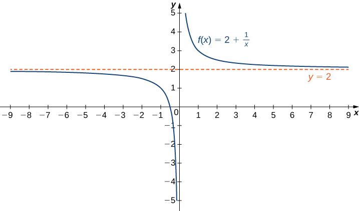
| [latex]x[/latex] | [latex]10[/latex] | [latex]100[/latex] | [latex]1,000[/latex] | [latex]10,000[/latex] |
| [latex]2+\frac{1}{x}[/latex] | [latex]2.1[/latex] | [latex]2.01[/latex] | [latex]2.001[/latex] | [latex]2.0001[/latex] |
| [latex]x[/latex] | [latex]-10[/latex] | [latex]-100[/latex] | [latex]-1000[/latex] | [latex]-10,000[/latex] |
| [latex]2+\frac{1}{x}[/latex] | [latex]1.9[/latex] | [latex]1.99[/latex] | [latex]1.999[/latex] | [latex]1.9999[/latex] |
More generally, for any function [latex]f[/latex], we say the limit as [latex]x \to \infty[/latex] of [latex]f(x)[/latex] is [latex]L[/latex] if [latex]f(x)[/latex] becomes arbitrarily close to [latex]L[/latex] as long as [latex]x[/latex] is sufficiently large. In that case, we write:
[latex]\underset{x\to \infty}{\lim}f(x)=L[/latex].
Similarly, we say the limit as [latex]x\to −\infty[/latex] of [latex]f(x)[/latex] is [latex]L[/latex] if [latex]f(x)[/latex] becomes arbitrarily close to [latex]L[/latex] as long as [latex]x<0[/latex] and [latex]|x|[/latex] is sufficiently large. In that case, we write:
[latex]\underset{x\to −\infty }{\lim}f(x)=L[/latex].
We now look at the definition of a function having a limit at infinity.
limit at infinity (informal)
If the values of [latex]f(x)[/latex] become arbitrarily close to [latex]L[/latex] as [latex]x[/latex] becomes sufficiently large, we say the function [latex]f[/latex] has a limit at infinity and write:
If the values of [latex]f(x)[/latex] becomes arbitrarily close to [latex]L[/latex] for [latex]x<0[/latex] as [latex]|x|[/latex] becomes sufficiently large, we say that the function [latex]f[/latex] has a limit at negative infinity and write:
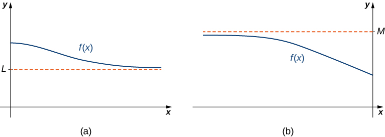
If the values [latex]f(x)[/latex] are getting arbitrarily close to some finite value [latex]L[/latex] as [latex]x\to \infty[/latex] or [latex]x\to −\infty[/latex], the graph of [latex]f[/latex] approaches the line [latex]y=L[/latex]. In that case, the line [latex]y=L[/latex] is a horizontal asymptote of [latex]f[/latex].
For the function [latex]f(x)=\frac{1}{x}[/latex], since [latex]\underset{x\to \infty }{\lim}f(x)=0[/latex], the line [latex]y=0[/latex] is a horizontal asymptote of [latex]f(x)=\frac{1}{x}[/latex].
horizontal asymptote
If [latex]\underset{x\to \infty }{\lim}f(x)=L[/latex] or [latex]\underset{x \to −\infty}{\lim}f(x)=L[/latex], we say the line [latex]y=L[/latex] is a horizontal asymptote of [latex]f[/latex].
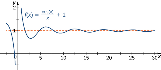
A function cannot cross a vertical asymptote because the graph must approach infinity (or negative infinity) from at least one direction as [latex]x[/latex] approaches the vertical asymptote. However, a function may cross a horizontal asymptote. In fact, a function may cross a horizontal asymptote an unlimited number of times.
The function [latex]f(x)=\frac{ \cos x}{x}+1[/latex] shown below intersects the horizontal asymptote [latex]y=1[/latex] an infinite number of times as it oscillates around the asymptote with ever-decreasing amplitude.
The algebraic limit laws and squeeze theorem we introduced earlier also apply to limits at infinity. We illustrate how to use these laws to compute several limits at infinity.
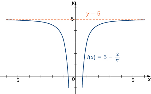
For each of the following functions [latex]f[/latex], evaluate [latex]\underset{x\to \infty }{\lim}f(x)[/latex] and [latex]\underset{x\to −\infty }{\lim}f(x)[/latex]. Determine the horizontal asymptote(s) for [latex]f[/latex].
- [latex]f(x)=5-\frac{2}{x^2}[/latex]
- [latex]f(x)=\dfrac{\sin x}{x}[/latex]
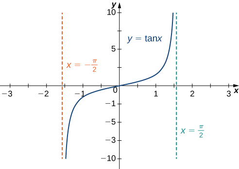
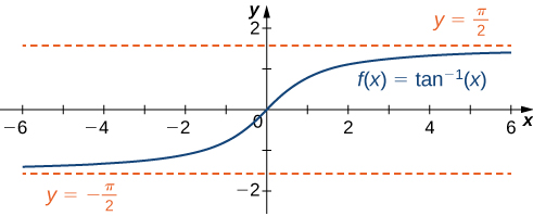
- [latex]f(x)= \tan^{-1} (x)[/latex]

Infinite Limits at Infinity
Sometimes the values of a function [latex]f[/latex] become arbitrarily large as [latex]x\to \infty[/latex] (or as [latex]x\to −\infty )[/latex]. In this case, we write [latex]\underset{x\to \infty }{\lim}f(x)=\infty[/latex] (or [latex]\underset{x\to −\infty }{\lim}f(x)=\infty )[/latex].
On the other hand, if the values of [latex]f[/latex] are negative but become arbitrarily large in magnitude as [latex]x\to \infty[/latex] (or as [latex]x\to −\infty )[/latex], we write [latex]\underset{x\to \infty }{\lim}f(x)=−\infty[/latex] (or [latex]\underset{x\to −\infty }{\lim}f(x)=−\infty )[/latex].
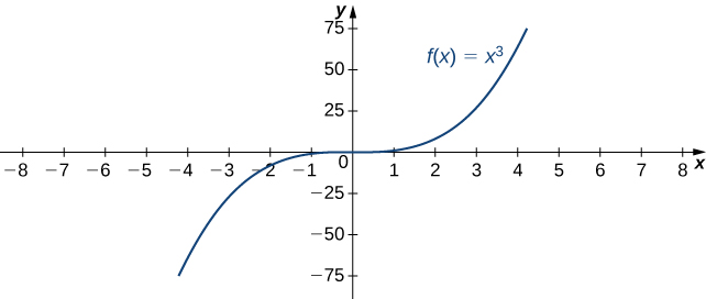
Consider the function [latex]f(x)=x^3[/latex].
| [latex]x[/latex] | [latex]10[/latex] | [latex]20[/latex] | [latex]50[/latex] | [latex]100[/latex] | [latex]1000[/latex] |
| [latex]x^3[/latex] | [latex]1000[/latex] | [latex]8000[/latex] | [latex]125,000[/latex] | [latex]1,000,000[/latex] | [latex]1,000,000,000[/latex] |
| [latex]x[/latex] | [latex]-10[/latex] | [latex]-20[/latex] | [latex]-50[/latex] | [latex]-100[/latex] | [latex]-1000[/latex] |
| [latex]x^3[/latex] | [latex]-1000[/latex] | [latex]-8000[/latex] | [latex]-125,000[/latex] | [latex]-1,000,000[/latex] | [latex]-1,000,000,000[/latex] |
As seen in the table and figure above, as [latex]x\to \infty[/latex] the values [latex]f(x)[/latex] become arbitrarily large. Therefore, [latex]\underset{x\to \infty }{\lim}x^3=\infty[/latex].
On the other hand, as [latex]x\to −\infty[/latex], the values of [latex]f(x)=x^3[/latex] are negative but become arbitrarily large in magnitude. Consequently, [latex]\underset{x\to −\infty }{\lim}x^3=−\infty[/latex].
infinite limits at infinity (informal)
We say a function [latex]f[/latex] has an infinite limit at infinity and write:
if [latex]f(x)[/latex] becomes arbitrarily large for [latex]x[/latex] sufficiently large. We say a function has a negative infinite limit at infinity and write:
if [latex]f(x)<0[/latex] and [latex]|f(x)|[/latex] becomes arbitrarily large for [latex]x[/latex] sufficiently large.
Similarly, we can define infinite limits as [latex]x\to −\infty[/latex].