Graphing Inverse Functions
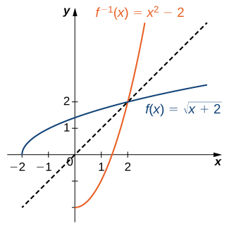
Let’s consider the relationship between the graph of a function [latex]f[/latex] and the graph of its inverse.
Consider the graph of [latex]f[/latex] shown in Figure 9(a) and a point [latex](a,b)[/latex] on the graph.
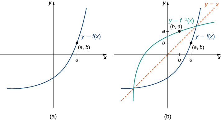
Since [latex]b=f(a)[/latex], then [latex]f^{-1}(b)=a[/latex]. Therefore, when we graph [latex]f^{-1}[/latex], the point [latex](b,a)[/latex] is on the graph. As a result, the graph of [latex]f^{-1}[/latex] is a reflection of the graph of [latex]f[/latex] about the line [latex]y=x[/latex].
How to: Graph the Inverse of a Function
- Plot the Function: Graph the original function [latex]f(x)[/latex] and plot a few key points.
- Reflect Over Line: Reflect these points over the line [latex]y=x[/latex] to find the corresponding points on [latex]f^{-1}[/latex].
- Draw the Inverse: Connect these reflected points to graph the inverse function.
- Check: Ensure that each point [latex](a,b)[/latex] on the original function corresponds to the point [latex](b,a)[/latex] on the inverse function.
- Line of Symmetry: The line [latex]y=x[/latex] should act as a line of symmetry between the function and its inverse.
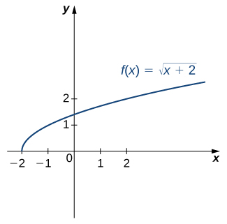
For the graph of [latex]f[/latex] in the following image, sketch a graph of [latex]f^{-1}[/latex] by sketching the line [latex]y=x[/latex] and using symmetry. Identify the domain and range of [latex]f^{-1}[/latex].
Restricting Domains
As we have seen, [latex]f(x)=x^2[/latex] does not have an inverse function because it is not one-to-one. However, we can choose a subset of the domain of [latex]f[/latex] such that the function is one-to-one. This subset is called a restricted domain.
By restricting the domain of [latex]f[/latex], we can define a new function [latex]g[/latex] such that the domain of [latex]g[/latex] is the restricted domain of [latex]f[/latex] and [latex]g(x)=f(x)[/latex] for all [latex]x[/latex] in the domain of [latex]g[/latex]. Then we can define an inverse function for [latex]g[/latex] on that domain.
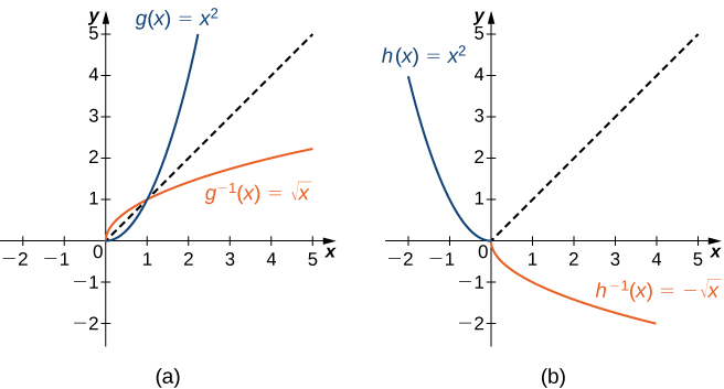
For example, since [latex]f(x)=x^2[/latex] is one-to-one on the interval [latex][0,\infty)[/latex], we can define a new function [latex]g[/latex] such that the domain of [latex]g[/latex] is [latex][0,\infty)[/latex] and [latex]g(x)=x^2[/latex] for all [latex]x[/latex] in its domain. Since [latex]g[/latex] is a one-to-one function, it has an inverse function, given by the formula [latex]g^{-1}(x)=\sqrt{x}[/latex].
On the other hand, the function [latex]f(x)=x^2[/latex] is also one-to-one on the domain [latex](−\infty,0][/latex]. Therefore, we could also define a new function [latex]h[/latex] such that the domain of [latex]h[/latex] is [latex](−\infty,0][/latex] and [latex]h(x)=x^2[/latex] for all [latex]x[/latex] in the domain of [latex]h[/latex]. Then [latex]h[/latex] is a one-to-one function and must also have an inverse. Its inverse is given by the formula [latex]h^{-1}(x)=−\sqrt{x}[/latex] (Figure 13).
restricted domain
Some functions don’t have inverses over their full domains because they’re not one-to-one. By restricting the domain, we ensure the function is one-to-one. Once the domain is restricted, we can define an inverse.
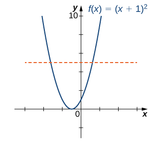
Consider the function [latex]f(x)=(x+1)^2[/latex].
- Sketch the graph of [latex]f[/latex] and use the horizontal line test to show that [latex]f[/latex] is not one-to-one.
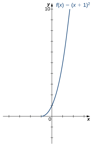
- Show that [latex]f[/latex] is one-to-one on the restricted domain [latex][-1,\infty)[/latex]. Determine the domain and range for the inverse of [latex]f[/latex] on this restricted domain and find a formula for [latex]f^{-1}[/latex].