- Check if a function can have an inverse by using the horizontal line test
- Determine a function’s inverse and draw its mirrored graph
- Calculate values using inverse trig functions like arcsine, arccosine, and arctangent
Inverse Functions
An inverse function reverses the operation done by a particular function. In other words, whatever a function does, the inverse function undoes it. If we have a function [latex]f[/latex] that takes an input [latex]x[/latex] and produces an output [latex]f(x)[/latex], the inverse function, denoted as [latex]f^{−1}[/latex], takes [latex]f(x)[/latex] as its input and returns the original [latex]x[/latex] as its output.
inverse functions
An inverse function reverses the effect of the original function, effectively ‘undoing’ what the original function does.
The inverse of a function [latex]f[/latex] is denoted by [latex]f^{−1}[/latex].
Note that [latex]f^{-1}[/latex] is read as “f inverse.” Here, the [latex]-1[/latex] is not used as an exponent and [latex]f^{-1}(x) \ne \frac{1}{f(x)}[/latex].
For instance, let’s consider the function [latex]f(x)=x^3+4[/latex]. To find the inverse, we set [latex]y= f(x)[/latex], which gives us [latex]y=x^3+4[/latex]. We get the inverse function [latex]f^{−1}(y)[/latex] by solving for [latex]x[/latex].
In this instance, subtract [latex]4[/latex] from both sides to get [latex]t-4=x^3[/latex], and then take the cube root of both sides. This gives us [latex]x=\sqrt[3]{y-4}[/latex]. This equation defines [latex]x[/latex] as a function of [latex]y[/latex].
Denoting this function as [latex]f^{-1}[/latex], and writing [latex]x=f^{-1}(y)=\sqrt[3]{y-4}[/latex], we see that for any [latex]x[/latex] in the domain of [latex]f, \, f^{-1}(f(x))=f^{-1}(x^3+4)=x[/latex].
Thus, this new function, [latex]f^{-1}[/latex], “undid” what the original function [latex]f[/latex] did.
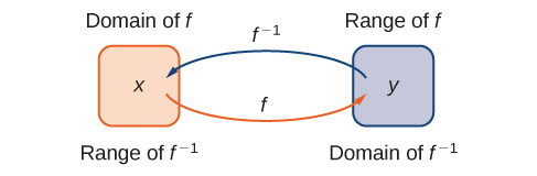
Two functions are inverses of each other if the domain [latex]D[/latex] of [latex]f[/latex] becomes the range [latex]R[/latex] of [latex]f^{−1}[/latex] and vice versa.
In other words, for a function [latex]f[/latex] and its inverse [latex]f^{-1}[/latex],
Figure 1 shows the relationship between the domain and range of [latex]f[/latex] and the domain and range of [latex]f^{-1}[/latex].
Horizontal Line Test
Not all functions have inverses that are also functions, because for a function to have an inverse, each output must be linked to one and only one input. This unique pairing ensures that the inverse process can always match an output back to one specific input, fulfilling the definition of a function.
For example, let’s try to find the inverse function for [latex]f(x)=x^2[/latex]. Solving the equation [latex]y=x^2[/latex] for [latex]x[/latex], we arrive at the equation [latex]x= \pm \sqrt{y}[/latex]. This equation does not describe [latex]x[/latex] as a function of [latex]y[/latex] because there are two solutions to this equation for every [latex]y>0[/latex].
The problem with trying to find an inverse function for [latex]f(x)=x^2[/latex] is that two inputs are sent to the same output for each output [latex]y>0[/latex]. The function [latex]f(x)=x^3+4[/latex] discussed earlier did not have this problem. For that function, each input was sent to a different output.
A function that sends each input to a different output is called a one-to-one function.
one-to-one
A one-to-one function is a type of function in which each output value is paired with a unique input value.
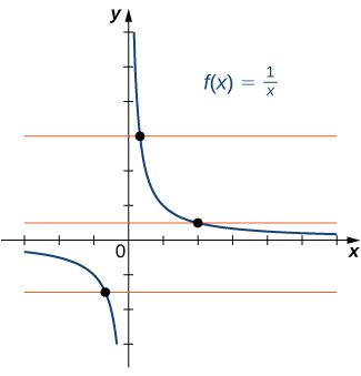
One way to determine whether a function is one-to-one is by looking at its graph. If a function is one-to-one, then no two inputs can be sent to the same output. Therefore, if we draw a horizontal line anywhere in the [latex]xy[/latex]-plane, it cannot intersect the graph more than once. This is known as the horizontal line test.
Horizontal Line Test
A function [latex]f[/latex] is one-to-one, if and only if, every horizontal line intersects the graph of [latex]f[/latex] no more than once.
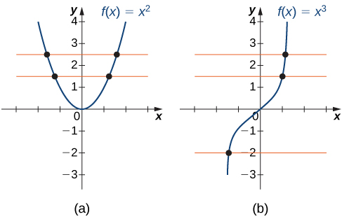
Note that the horizontal line test is different from the vertical line test. The vertical line test determines whether a graph is the graph of a function. The horizontal line test determines whether a function is one-to-one (Figure 3).
The Vertical Line Test
The vertical line test confirms whether a relation is a function by checking that every vertical line crosses the graph at most once.
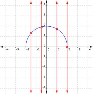
When a vertical line is placed across the plot of this relation, it does not intersect the graph more than once for any values of [latex]x[/latex]. This is a graph of a function.
If, on the other hand, a graph shows two or more intersections with a vertical line, then an input ([latex]x[/latex]-coordinate) can have more than one output ([latex]y[/latex]-coordinate), and [latex]y[/latex] is not a function of [latex]x[/latex].
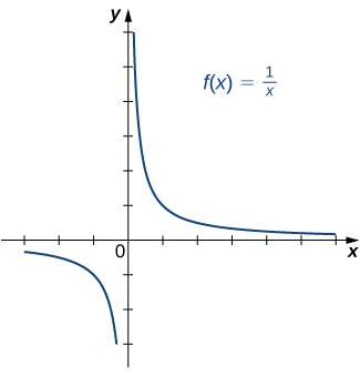
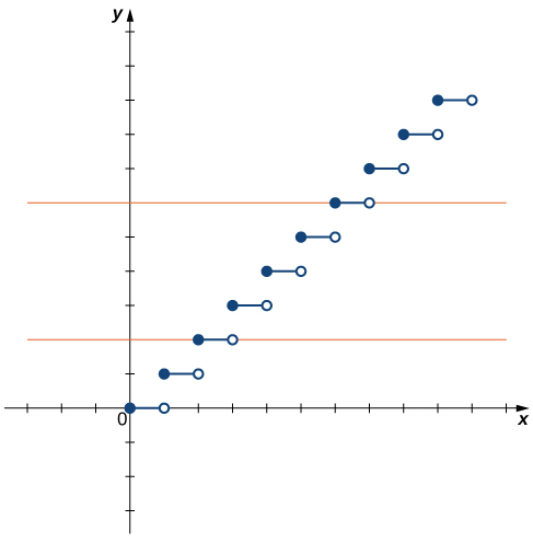
For each of the following functions, use the horizontal line test to determine whether it is one-to-one.
a.
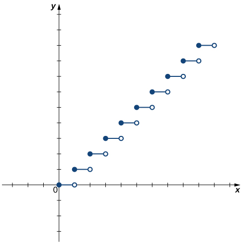
b.