The Definition of a Limit Cont.

Estimating Limits Using Graphs

At this point, we see from the tables that it may be just as easy, if not easier, to estimate a limit of a function by inspecting its graph as it is to estimate the limit by using a table of functional values.

In the example below, we evaluate a limit exclusively by looking at a graph rather than by using a table of functional values. 

For [latex]g(x)[/latex] shown in the figure below, evaluate [latex]\underset{x\to -1}{\lim}g(x)[/latex].

Show Solution

Despite the fact that [latex]g(-1)=4[/latex], as the [latex]x[/latex]-values approach [latex]−1[/latex] from either side, the [latex]g(x)[/latex] values approach [latex]3[/latex]. Therefore, [latex]\underset{x\to -1}{\lim}g(x)=3[/latex].

Note that we can determine this limit without even knowing the algebraic expression of the function.

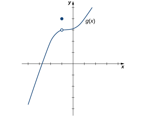
Based on the example above, we make the following observation: It is possible for the limit of a function to exist at a point, and for the function to be defined at this point, but the limit of the function and the value of the function at the point may be different.

Exploring the Limits: Beyond Tables and Graphs

Analyzing functional values in tables or observing a function’s graph can offer initial insights into its limit at a particular point. However, these approaches often involve a degree of estimation.

To gain a more precise understanding, we’ll move towards algebraic methods for evaluating limits. Before we delve into these methods in the following section, we’ll introduce two essential limits that underpin the forthcoming algebraic techniques.

We can make the following observations about these two limits.

1. For the first limit, observe that as [latex]x[/latex] approaches [latex]a[/latex], so does [latex]f(x)[/latex], because [latex]f(x)=x[/latex]. Consequently, [latex]\underset{x\to a}{\lim}x=a[/latex].
2. For the second limit, consider the table below.

Observe that for all values of [latex]x[/latex] (regardless of whether they are approaching [latex]a[/latex]), the values [latex]f(x)[/latex] remain constant at [latex]c[/latex]. We have no choice but to conclude [latex]\underset{x\to a}{\lim}c=c[/latex].

The Existence of a Limit

Understanding when a limit exists is fundamental to grasping the behavior of functions as their inputs approach a specific value.

A limit is considered to exist at a certain point if the function values converge to a single, real number as we near that point from any direction. This behavior is indicative of the function’s stability near the point of interest.

If, instead, the function values diverge or oscillate without settling on a single value, we say the limit at that point does not exist.

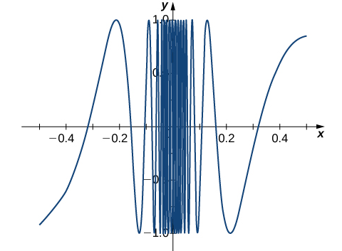
The upcoming example illustrates this concept by examining a scenario where a limit fails to exist

Mathematicians frequently abbreviate “does not exist” as DNE.

Evaluate [latex]\underset{x\to 0}{\lim} \sin \left(\dfrac{1}{x}\right)[/latex] using a table of values.

Show Solution

The table below lists values for the function [latex]\sin \left(\dfrac{1}{x}\right)[/latex] for the given values of [latex]x[/latex].

Table of Functional Values for [latex]\underset{x\to 0}{\lim} \sin (\frac{1}{x})[/latex]

[latex]x[/latex]	[latex]\sin (\frac{1}{x})[/latex]		[latex]x[/latex]	[latex]\sin (\frac{1}{x})[/latex]
[latex]−0.1[/latex]	[latex]0.544021110889[/latex]		[latex]0.1[/latex]	[latex]−0.544021110889[/latex]
[latex]−0.01[/latex]	[latex]0.50636564111[/latex]		[latex]0.01[/latex]	[latex]−0.50636564111[/latex]
[latex]−0.001[/latex]	[latex]−0.8268795405312[/latex]		[latex]0.001[/latex]	[latex]0.826879540532[/latex]
[latex]−0.0001[/latex]	[latex]0.305614388888[/latex]		[latex]0.0001[/latex]	[latex]−0.305614388888[/latex]
[latex]−0.00001[/latex]	[latex]−0.035748797987[/latex]		[latex]0.00001[/latex]	[latex]0.035748797987[/latex]
[latex]−0.000001[/latex]	[latex]0.349993504187[/latex]		[latex]0.000001[/latex]	[latex]−0.349993504187[/latex]

After examining the table of functional values, we can see that the [latex]y[/latex]-values do not seem to approach any one single value. It appears the limit does not exist. Before drawing this conclusion, let’s take a more systematic approach. Take the following sequence of [latex]x[/latex]-values approaching 0:

[latex]\frac{2}{\pi }, \, \frac{2}{3\pi }, \, \frac{2}{5\pi }, \, \frac{2}{7\pi }, \, \frac{2}{9\pi }, \, \frac{2}{11\pi }, \, \cdots[/latex]

The corresponding [latex]y[/latex]-values are

[latex]1, \, -1, \, 1, \, -1, \, 1, \, -1, \, \cdots[/latex]

At this point we can indeed conclude that [latex]\underset{x\to 0}{\lim} \sin (\frac{1}{x})[/latex] does not exist.

Thus, we would write [latex]\underset{x\to 0}{\lim} \sin (\frac{1}{x})[/latex] DNE.

The graph of [latex]f(x)= \sin (\frac{1}{x})[/latex] is shown in Figure 6 and it gives a clearer picture of the behavior of [latex]\sin (\frac{1}{x})[/latex] as [latex]x[/latex] approaches [latex]0[/latex]. You can see that [latex]\sin (\frac{1}{x})[/latex] oscillates ever more wildly between [latex]−1[/latex] and [latex]1[/latex] as [latex]x[/latex] approaches [latex]0[/latex].