Approximating Areas
-
- They are equal; both represent the sum of the first [latex]10[/latex] whole numbers.
- They are equal; both represent the sum of the first [latex]10[/latex] whole numbers.
- They are equal by substituting [latex]j=i-1[/latex].
- They are equal; the first sum factors the terms of the second.
- [latex]385-30=355[/latex]
- [latex]15-(-12)=27[/latex]
- [latex]5(15)+4(-12)=27[/latex]
- [latex]\underset{j=1}{\overset{50}{\Sigma}} j^2-2\underset{j=1}{\overset{50}{\Sigma}} j=\frac{(50)(51)(101)}{6}-\frac{2(50)(51)}{2}=40,375[/latex]
- [latex]4\underset{k=1}{\overset{25}{\Sigma}} k^2-100\underset{k=1}{\overset{25}{\Sigma}} k=\frac{4(25)(26)(51)}{9}-50(25)(26)=-10,400[/latex]
- [latex]R_4=0.25[/latex]
- [latex]R_6=0.372[/latex]
- [latex]L_4=2.20[/latex]
- [latex]L_8=0.6875[/latex]
- [latex]L_{10}=\frac{4}{10}\underset{i=1}{\overset{10}{\Sigma}} \sqrt{4-(-2+4\frac{(i-1)}{10})}[/latex]
- [latex]R_{100}=\frac{e-1}{100}\underset{i=1}{\overset{100}{\Sigma}} \ln (1+(e-1)\frac{i}{100})[/latex]
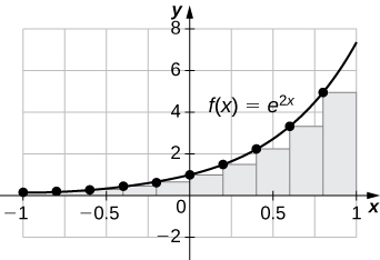
![A graph of the given function on the interval [0, 1]. It is set up for a left endpoint approximation and is an underestimate because the function is increasing. Ten rectangles are shown for visual clarity, but this behavior persists for more rectangles.](https://s3-us-west-2.amazonaws.com/courses-images/wp-content/uploads/sites/2332/2018/01/11203930/CNX_Calc_Figure_05_01_207.jpg)
[latex]R_{100}=0.33835, \, L_{100}=0.32835[/latex]. The plot shows that the left Riemann sum is an underestimate because the function is increasing. Similarly, the right Riemann sum is an overestimate. The area lies between the left and right Riemann sums. Ten rectangles are shown for visual clarity. This behavior persists for more rectangles.
![A graph of the given function over [-1,1] set up for a left endpoint approximation. It is an underestimate since the function is increasing. Ten rectangles are shown for visual clarity, but this behavior persists for more rectangles.](https://s3-us-west-2.amazonaws.com/courses-images/wp-content/uploads/sites/2332/2018/01/11203933/CNX_Calc_Figure_05_01_209.jpg)
[latex]L_{100}=-0.02, \, R_{100}=0.02[/latex]. The left endpoint sum is an underestimate because the function is increasing. Similarly, a right endpoint approximation is an overestimate. The area lies between the left and right endpoint estimates.
[latex]L_{100}=3.555, \, R_{100}=3.670[/latex]. The plot shows that the left Riemann sum is an underestimate because the function is increasing. Ten rectangles are shown for visual clarity. This behavior persists for more rectangles.
- [latex]L_6=9.000=R_6[/latex]. The graph of [latex]f[/latex] is a triangle with area [latex]9[/latex].
- [latex]L_6=13.12899=R_6[/latex]. They are equal.
- The sum represents the cumulative rainfall in January 2009.
- The total mileage is [latex]7 \times \underset{i=1}{\overset{25}{\Sigma}} (1+\frac{(i-1)}{10})=7 \times 25+\frac{7}{10} \times 12 \times 25=385[/latex] mi.
- Add the numbers to get [latex]8.1[/latex]-in. net increase.
- [latex]309,389,957[/latex]
- [latex]L_8=3+2+1+2+3+4+5+4=24[/latex]
- [latex]L_8=3+5+7+6+8+6+5+4=44[/latex]
The Definite Integral
- [latex]\displaystyle\int_0^2 (5x^2-3x^3) dx[/latex]
- [latex]\displaystyle\int_0^1 \cos^2 (2\pi x) dx[/latex]
- [latex]\displaystyle\int_0^1 x dx[/latex]
- [latex]\displaystyle\int_3^6 x dx[/latex]
- [latex]\displaystyle\int_1^2 x\log(x^2) dx[/latex]
- [latex]1+2 \cdot 2+3 \cdot 3=14[/latex]
- [latex]1-4+9=6[/latex]
- [latex]1-2\pi +9=10-2\pi[/latex]
- The integral is the area of the triangle, [latex]\frac{1}{2}[/latex]
- The integral is the area of the triangle, [latex]9[/latex].
- The integral is the area [latex]\frac{1}{2}\pi r^2=2\pi[/latex].
- The integral is the area of the “big” triangle minus the “missing” triangle, [latex]9-\frac{1}{2}[/latex].
- [latex]L=2+0+10+5+4=21,R=0+10+10+2+0=22, \, \frac{L+R}{2}=21.5[/latex]
- [latex]L=0+4+0+4+2=10,R=4+0+2+4+0=10, \, \frac{L+R}{2}=10[/latex]
- [latex]\displaystyle\int_2^4 f(x) dx + \displaystyle\int_2^4 g(x) dx=8-3=5[/latex]
- [latex]\displaystyle\int_2^4 f(x) dx - \displaystyle\int_2^4 g(x) dx=8+3=11[/latex]
- [latex]4 \displaystyle\int_2^4 f(x) dx - 3 \displaystyle\int_2^4 g(x) dx = 32+9=41[/latex]
- The integrand is odd; the integral is zero.
- The integrand is antisymmetric with respect to [latex]x=3[/latex]. The integral is zero.
- [latex]1-\frac{1}{2}+\frac{1}{3}-\frac{1}{4}=\frac{7}{12}[/latex]
- [latex]\displaystyle\int_0^1 (1-6x+12x^2-8x^3) dx = (x-3x^{2}+4x^{3}-2x^{4})=(1-3+4-2)=0[/latex]
- [latex]7-\frac{5}{4}=\frac{23}{4}[/latex]
- The integrand is negative over [latex][-2,3][/latex].
- [latex]x \le x^2[/latex] over [latex][1,2][/latex], so [latex]\sqrt{1+x} \le \sqrt{1+x^2}[/latex] over [latex][1,2][/latex].
- [latex]\cos (t) \ge \frac{\sqrt{2}}{2}[/latex]. Multiply by the length of the interval to get the inequality.
- [latex]f_{\text{ave}}=0; \, c=0[/latex]
- [latex]\frac{3}{2}[/latex] when [latex]c= \pm \frac{3}{2}[/latex]
- [latex]f_{\text{ave}}=0; \, c=\frac{\pi}{2},\frac{3\pi}{2}[/latex]
- [latex]L_{100}=1.294, \, R_{100}=1.301[/latex]; the exact average is between these values.
- [latex]L_{100} \times (\frac{1}{2})=0.5178, \, R_{100} \times (\frac{1}{2})=0.5294[/latex]
- [latex]L_1=0, \, L_{10} \times (\frac{1}{2})=8.743493, \, L_{100} \times (\frac{1}{2})=12.861728[/latex]. The exact answer [latex]\approx 26.799[/latex], so [latex]L_{100}[/latex] is not accurate.
- [latex]L_1 \times (\frac{1}{\pi})=1.352, \, L_{10} \times (\frac{1}{\pi})=-0.1837, \, L_{100} \times (\frac{1}{\pi})=-0.2956[/latex]. The exact answer [latex]\approx -0.303[/latex], so [latex]L_{100}[/latex] is not accurate to first decimal.
- Use [latex]\tan^2 \theta +1= \sec^2 \theta[/latex]. Then, [latex]B-A=\displaystyle\int_{−\pi/4}^{\pi/4} 1 dx = \frac{\pi}{2}[/latex].
The Fundamental Theorem of Calculus
- [latex]{e}^{ \cos t}[/latex]
- [latex]\frac{1}{\sqrt{16-{x}^{2}}}[/latex]
- [latex]\sqrt{x}\frac{d}{dx}\sqrt{x}=\frac{1}{2}[/latex]
- [latex]\text{−}\sqrt{1-{ \cos }^{2}x}\frac{d}{dx} \cos x=| \sin x| \sin x[/latex]
- [latex]2x\frac{|x|}{1+{x}^{2}}[/latex]
- [latex]\text{ln}({e}^{2x})\frac{d}{dx}{e}^{x}=2x{e}^{x}[/latex]
-
- [latex]f[/latex] is positive over [latex]\left[1,2\right][/latex] and [latex]\left[5,6\right],[/latex] negative over [latex]\left[0,1\right][/latex] and [latex]\left[3,4\right],[/latex] and zero over [latex]\left[2,3\right][/latex] and [latex]\left[4,5\right].[/latex]
- The maximum value is [latex]2[/latex] and the minimum is −[latex]3[/latex].
- The average value is [latex]0[/latex].
-
- ℓ is positive over [latex]\left[0,1\right][/latex] and [latex]\left[3,6\right],[/latex] and negative over [latex]\left[1,3\right].[/latex]
- It is increasing over [latex]\left[0,1\right][/latex] and [latex]\left[3,5\right],[/latex] and it is constant over [latex]\left[1,3\right][/latex] and [latex]\left[5,6\right].[/latex]
- Its average value is [latex]\frac{1}{3}.[/latex]
- [latex]{T}_{10}=49.08,{\displaystyle\int }_{-2}^{3}{x}^{3}+6{x}^{2}+x-5dx=48[/latex]
- [latex]{T}_{10}=260.836,{\displaystyle\int }_{1}^{9}(\sqrt{x}+{x}^{2})dx=260[/latex]
- [latex]{T}_{10}=3.058,{\displaystyle\int }_{1}^{4}\frac{4}{{x}^{2}}dx=3[/latex]
- [latex]F(x)=\frac{{x}^{3}}{3}+\frac{3{x}^{2}}{2}-5x,F(3)-F(-2)=-\frac{35}{6}[/latex]
- [latex]F(x)=-\frac{{t}^{5}}{5}+\frac{13{t}^{3}}{3}-36t,F(3)-F(2)=\frac{62}{15}[/latex]
- [latex]F(x)=\frac{{x}^{100}}{100},F(1)-F(0)=\frac{1}{100}[/latex]
- [latex]F(x)=\frac{{x}^{3}}{3}+\frac{1}{x},F(4)-F(\frac{1}{4})=\frac{1125}{64}[/latex]
- [latex]F(x)=\sqrt{x},F(4)-F(1)=1[/latex
- [latex]F(x)=\frac{4}{3}{t}^{3\text{/}4},F(16)-F(1)=\frac{28}{3}[/latex]
- [latex]F(x)=\text{−} \cos x,F(\frac{\pi }{2})-F(0)=1[/latex]
- [latex]F(x)= \sec x,F(\frac{\pi }{4})-F(0)=\sqrt{2}-1[/latex]
- [latex]F(x)=\text{−} \cot (x),F(\frac{\pi }{2})-F(\frac{\pi }{4})=1[/latex]
- [latex]F(x)=-\frac{1}{x}+\frac{1}{2{x}^{2}},F(-1)-F(-2)=\frac{7}{8}[/latex]
- [latex]F(x)={e}^{x}-e[/latex]
- [latex]F(x)=0[/latex]
- [latex]{\displaystyle\int }_{-2}^{-1}({t}^{2}-2t-3)dt-{\displaystyle\int }_{-1}^{3}({t}^{2}-2t-3)dt+{\displaystyle\int }_{3}^{4}({t}^{2}-2t-3)dt=\frac{46}{3}[/latex]
- [latex]\text{−}{\displaystyle\int }_{\text{−}\pi \text{/}2}^{0} \sin tdt+{\displaystyle\int }_{0}^{\pi \text{/}2} \sin tdt=2[/latex]
-
- The average is [latex]11.21×{10}^{9}[/latex] since [latex]\cos (\frac{\pi t}{6})[/latex] has period [latex]12[/latex] and integral [latex]0[/latex] over any period. Consumption is equal to the average when [latex]\cos (\frac{\pi t}{6})=0,[/latex] when [latex]t=3,[/latex] and when [latex]t=9.[/latex]
- Total consumption is the average rate times duration: [latex]11.21×12×{10}^{9}=1.35×{10}^{11}[/latex]
- [latex]{10}^{9}(11.21-\frac{1}{6}{\displaystyle\int }_{3}^{9} \cos (\frac{\pi t}{6})dt)={10}^{9}(11.21+\frac{2}{\pi })=11.84x{10}^{9}[/latex]
- If [latex]f[/latex] is not constant, then its average is strictly smaller than the maximum and larger than the minimum, which are attained over [latex]\left[a,b\right][/latex] by the extreme value theorem.
-
- [latex]{d}^{2}\theta ={(a \cos \theta +c)}^{2}+{b}^{2}{ \sin }^{2}\theta ={a}^{2}+{c}^{2}{ \cos }^{2}\theta +2ac \cos \theta ={(a+c \cos \theta )}^{2};[/latex]
- [latex]\overline{d}=\frac{1}{2\pi }{\displaystyle\int }_{0}^{2\pi }(a+2c \cos \theta )d\theta =a[/latex]
- Mean gravitational force = [latex]\frac{GmM}{2}{\displaystyle\int }_{0}^{2\pi }\frac{1}{{(a+2\sqrt{{a}^{2}-{b}^{2}} \cos \theta )}^{2}}d\theta .[/latex]
Integration Formulas and the Net Change Theorem
- [latex]\displaystyle\int (\sqrt{x}-\frac{1}{\sqrt{x}})dx=\int {x}^{1\text{/}2}dx-\int {x}^{-1\text{/}2}dx=\frac{2}{3}{x}^{3\text{/}2}+{C}_{1}-2{x}^{1\text{/}2}+{C}_{2}=\frac{2}{3}{x}^{3\text{/}2}-2{x}^{1\text{/}2}+C[/latex]
- [latex]\displaystyle\int \frac{dx}{2x}=\frac{1}{2}\text{ln}|x|+C[/latex]
- [latex]{\int }_{0}^{\pi } \sin xdx-{\int }_{0}^{\pi } \cos xdx=\text{−} \cos x{|}_{0}^{\pi }-( \sin x){|}_{0}^{\pi }=(\text{−}(-1)+1)-(0-0)=2[/latex]
- [latex]P(s)=4s,[/latex] so [latex]\frac{dP}{ds}=4[/latex] and [latex]{\int }_{2}^{4}4ds=8.[/latex]
- [latex]{\int }_{1}^{2}Nds=N[/latex]
- With [latex]p[/latex] as in the previous exercise, each of the [latex]12[/latex] pentagons increases in area from [latex]2p[/latex] to [latex]4p[/latex] units so the net increase in the area of the dodecahedron is [latex]36p[/latex] units.
- [latex]18{s}^{2}=6{\int }_{s}^{2s}2xdx[/latex]
- [latex]12\pi {R}^{2}=8\pi {\int }_{R}^{2R}rdr[/latex]
- Suppose that a particle moves along a straight line with velocity [latex]v(t)=4-2t,[/latex] where [latex]0\le t\le 2[/latex] (in meters per second). Find the displacement at time [latex]t[/latex] and the total distance traveled up to [latex]t=2.[/latex][latex]d(t)={\int }_{0}^{t}v(s)ds=4t-{t}^{2}.[/latex] The total distance is [latex]d(2)=4\text{m}\text{.}[/latex]
- [latex]d(t)={\displaystyle\int _{0}^{t}}v(s)ds.[/latex] For [latex]t<3,d(t)={\displaystyle\int _{0}^{t}}(6-2t)dt=6t-{t}^{2}.[/latex] For [latex]t>3,d(t)=d(3)+{\displaystyle\int _{3}^{t}}(2t-6)dt=18+({t}^{2}-6t).[/latex] The total distance is [latex]d(6)=18\text{m}\text{.}[/latex]
- [latex]v(t)=40-9.8t;h(t)=1.5+40t-4.9{t}^{2}[/latex] m/s
- The net increase is 1 unit.
- At [latex]t=5,[/latex] the height of water is [latex]x={(\frac{15}{\pi })}^{1\text{/}3}\text{m}\text{.}.[/latex] The net change in height from [latex]t=5[/latex] to [latex]t=10[/latex] is [latex]{(\frac{30}{\pi })}^{1\text{/}3}-{(\frac{15}{\pi })}^{1\text{/}3}[/latex] m.
- The total daily power consumption is estimated as the sum of the hourly power rates, or [latex]911[/latex] gW-h.
- [latex]17[/latex] kJ
-
- [latex]54.3\%[/latex]
- [latex]27.00\%[/latex]
- The curve in the following plot is [latex]2.35(t+3){e}^{-0.15(t+3)}.[/latex]
- In dry conditions, with initial velocity [latex]{v}_{0}=30[/latex] m/s, [latex]D=64.3[/latex] and, if [latex]{v}_{0}=25,D=44.64.[/latex] In wet conditions, if [latex]{v}_{0}=30,[/latex] and [latex]D=180[/latex] and if [latex]{v}_{0}=25,D=125.[/latex]
- 225 cal
- [latex]E(150)=28,E(300)=22,E(450)=16[/latex]
-
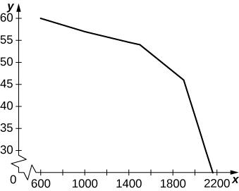
- Between 600 and 1000 the average decrease in vehicles per hour per lane is −[latex]0.0075[/latex]. Between [latex]1000[/latex] and [latex]1500[/latex] it is −[latex]0.006[/latex] per vehicles per hour per lane, and between [latex]1500[/latex] and [latex]2100[/latex] it is −[latex]0.04[/latex] vehicles per hour per lane.
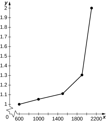 The graph is nonlinear, with minutes per mile increasing dramatically as vehicles per hour per lane reach [latex]2000[/latex].
- [latex]\frac{1}{40}{\int }_{0}^{40}(-0.068t+5.14)dt=-\frac{0.068(40)}{2}+5.14=3.78[/latex]