Approximating Areas

1. State whether the given sums are equal or unequal.
   1. [latex]\underset{i=1}{\overset{10}{\Sigma}} i[/latex] and [latex]\underset{k=1}{\overset{10}{\Sigma}} k[/latex]
   2. [latex]\underset{i=1}{\overset{10}{\Sigma}} i[/latex] and [latex]\underset{i=6}{\overset{15}{\Sigma}} (i-5)[/latex]
   3. [latex]\underset{i=1}{\overset{10}{\Sigma}} i(i-1)[/latex] and [latex]\underset{j=0}{\overset{9}{\Sigma}} (j+1)j[/latex]
   4. [latex]\underset{i=1}{\overset{10}{\Sigma}} i(i-1)[/latex] and [latex]\underset{k=1}{\overset{10}{\Sigma}}(k^2-k)[/latex]

In the following exercise, use the rules for sums of powers of integers to compute the sums.

2. [latex]\displaystyle\sum_{i=5}^{10} i^2[/latex]

Suppose that [latex]\underset{i=1}{\overset{100}{\Sigma}} a_i=15[/latex] and [latex]\underset{i=1}{\overset{100}{\Sigma}} b_i=-12[/latex]. In the following exercises (3-4), compute the sums.

3. [latex]\displaystyle\sum_{i=1}^{100} (a_i-b_i)[/latex]
4. [latex]\displaystyle\sum_{i=1}^{100} (5a_i+4b_i)[/latex]

In the following exercises (5-6), use summation properties and formulas to rewrite and evaluate the sums.

5. [latex]\displaystyle\sum_{j=1}^{50} (j^2-2j)[/latex]
6. [latex]\displaystyle\sum_{k=1}^{25} [(2k)^2-100k][/latex]

Let [latex]L_n[/latex] denote the left-endpoint sum using [latex]n[/latex] subintervals and let [latex]R_n[/latex] denote the corresponding right-endpoint sum. In the following exercises (7-10), compute the indicated left and right sums for the given functions on the indicated interval.

7. [latex]R_4[/latex] for [latex]g(x)= \cos (\pi x)[/latex] on [latex][0,1][/latex]
8. [latex]R_6[/latex] for [latex]f(x)=\dfrac{1}{x(x-1)}[/latex] on [latex][2,5][/latex]
9. [latex]L_4[/latex] for [latex]\dfrac{1}{x^2+1}[/latex] on [latex][-2,2][/latex]
10. [latex]L_8[/latex] for [latex]x^2-2x+1[/latex] on [latex][0,2][/latex]

Express the following endpoint sums in sigma notation but do not evaluate them (11-12).

11. [latex]L_{10}[/latex] for [latex]f(x)=\sqrt{4-x^2}[/latex] on [latex][-2,2][/latex]
12. [latex]R_{100}[/latex] for [latex]\ln x[/latex] on [latex][1,e][/latex]

In the following exercises (13-15), graph the function then use a calculator or a computer program to evaluate the following left and right endpoint sums. Is the area under the curve between the left and right endpoint sums?

13. [latex]L_{100}[/latex] and [latex]R_{100}[/latex] for [latex]y=x^2[/latex] on the interval [latex][0,1][/latex]
14. [latex]L_{100}[/latex] and [latex]R_{100}[/latex] for [latex]y=x^3[/latex] on the interval [latex][-1,1][/latex]
15. [latex]L_{100}[/latex] and [latex]R_{100}[/latex] for [latex]y=e^{2x}[/latex] on the interval [latex][-1,1][/latex]

For the following exercises (16-21), solve each problem.

16. Compute the left and right Riemann sums—[latex]L_6[/latex] and [latex]R_6[/latex], respectively—for [latex]f(x)=(3-|3-x|)[/latex] on [latex][0,6][/latex]. Compute their average value and compare it with the area under the graph of [latex]f[/latex].
17. Compute the left and right Riemann sums—[latex]L_6[/latex] and [latex]R_6[/latex], respectively—for [latex]f(x)=\sqrt{9-(x-3)^2}[/latex] on [latex][0,6][/latex] and compare their values.
18. Let [latex]r_j[/latex] denote the total rainfall in Portland on the [latex]j[/latex]th day of the year in 2009. Interpret [latex]\displaystyle\sum_{j=1}^{31} r_j[/latex].
19. To help get in shape, Joe gets a new pair of running shoes. If Joe runs [latex]1[/latex] mi each day in week 1 and adds [latex]\frac{1}{10}[/latex] mi to his daily routine each week, what is the total mileage on Joe’s shoes after [latex]25[/latex] weeks?
20. The following table gives the approximate increase in sea level in inches over [latex]20[/latex] years starting in the given year. Estimate the net change in mean sea level from 1870 to 2010.
    

    Approximate 20-Year Sea Level Increases, 1870–1990Source: http://link.springer.com/article/10.1007%2Fs10712-011-9119-1

    Starting Year	20-Year Change
    [latex]1870[/latex]	[latex]0.3[/latex]
    [latex]1890[/latex]	[latex]1.5[/latex]
    [latex]1910[/latex]	[latex]0.2[/latex]
    [latex]1930[/latex]	[latex]2.8[/latex]
    [latex]1950[/latex]	[latex]0.7[/latex]
    [latex]1970[/latex]	[latex]1.1[/latex]
    [latex]1990[/latex]	[latex]1.5[/latex]

21. The following table gives the percent growth of the U.S. population beginning in July of the year indicated. If the U.S. population was [latex]281,421,906[/latex] in July 2000, estimate the U.S. population in July 2010.
    

    Annual Percentage Growth of U.S. Population, 2000–2009Source: http://www.census.gov/popest/data.

    Year	% Change/Year
    [latex]2000[/latex]	[latex]1.12[/latex]
    [latex]2001[/latex]	[latex]0.99[/latex]
    [latex]2002[/latex]	[latex]0.93[/latex]
    [latex]2003[/latex]	[latex]0.86[/latex]
    [latex]2004[/latex]	[latex]0.93[/latex]
    [latex]2005[/latex]	[latex]0.93[/latex]
    [latex]2006[/latex]	[latex]0.97[/latex]
    [latex]2007[/latex]	[latex]0.96[/latex]
    [latex]2008[/latex]	[latex]0.95[/latex]
    [latex]2009[/latex]	[latex]0.88[/latex]

    Hint

    To obtain the population in July 2001, multiply the population in July 2000 by [latex]1.0112[/latex] to get [latex]284,573,831[/latex]

In the following exercises (22-23), estimate the areas under the curves by computing the left Riemann sums, [latex]L_8[/latex].

22. 
23. 

The Definite Integral

In the following exercises (1-5), express the limits as integrals.

1. [latex]\underset{n\to \infty }{\lim}\underset{i=1}{\overset{n}{\Sigma}}(5(x_i^*)^2-3(x_i^*)^3) \Delta x[/latex] over [latex][0,2][/latex]
2. [latex]\underset{n\to \infty }{\lim}\underset{i=1}{\overset{n}{\Sigma}} \cos^2 (2\pi x_i^*) \Delta x[/latex] over [latex][0,1][/latex]
3. [latex]R_n=\frac{1}{n}\underset{i=1}{\overset{n}{\Sigma}}\frac{i}{n}[/latex]
4. [latex]R_n=\frac{3}{n}\underset{i=1}{\overset{n}{\Sigma}}(3+3\frac{i}{n})[/latex]
5. [latex]R_n=\frac{1}{n}\underset{i=1}{\overset{n}{\Sigma}}(1+\frac{i}{n})\log((1+\frac{i}{n})^2)[/latex]

In the following exercises (6-8), evaluate the integrals of the functions graphed using the formulas for areas of triangles and circles, and subtracting the areas below the [latex]x[/latex]-axis.

6. 
7. 
8. 

In the following exercises (9-12), evaluate the integral using area formulas.

9. [latex]\displaystyle\int_2^3 (3-x) dx[/latex]
10. [latex]\displaystyle\int_0^6 (3-|x-3|) dx[/latex]
11. [latex]\displaystyle\int_1^5 \sqrt{4-(x-3)^2} dx[/latex]
12. [latex]\displaystyle\int_{-2}^3 (3-|x|) dx[/latex]

In the following exercises (13-14), use averages of values at the left ([latex]L[/latex]) and right ([latex]R[/latex]) endpoints to compute the integrals of the piecewise linear functions with graphs that pass through the given list of points over the indicated intervals.

13. [latex]\{(0,2),(1,0),(3,5),(5,5),(6,2),(8,0)\}[/latex] over [latex][0,8][/latex]
14. [latex]\{(-4,0),(-2,2),(0,0),(1,2),(3,2),(4,0)\}[/latex] over [latex][-4,4][/latex]

Suppose that [latex]\displaystyle\int_0^4 f(x) dx=5[/latex] and [latex]\displaystyle\int_0^2 f(x) dx=-3[/latex], and [latex]\displaystyle\int_0^4 g(x) dx=-1[/latex] and [latex]\displaystyle\int_0^2 g(x) dx=2[/latex]. In the following exercises (15-17), compute the integrals.

15. [latex]\displaystyle\int_2^4 (f(x)+g(x)) dx[/latex]
16. [latex]\displaystyle\int_2^4 (f(x)-g(x)) dx[/latex]
17. [latex]\displaystyle\int_2^4 (4f(x)-3g(x)) dx[/latex]

In the following exercises (18-19), use the identity [latex]\displaystyle\int_{−A}^A f(x) dx = \displaystyle\int_{−A}^0 f(x) dx + \displaystyle\int_0^A f(x) dx[/latex] to compute the integrals.

18. [latex]\displaystyle\int_{−\sqrt{\pi}}^{\sqrt{\pi}} \frac{t}{1+ \cos t} dt[/latex]
19. [latex]{\displaystyle\int }_{2}^{4}{(x-3)}^{3}dx[/latex] (Hint: Look at the graph of [latex]f[/latex].)

In the following exercises (20-22), given that [latex]\displaystyle\int_0^1 x dx = \frac{1}{2}, \, \displaystyle\int_0^1 x^2 dx = \frac{1}{3}[/latex], and [latex]\displaystyle\int_0^1 x^3 dx = \frac{1}{4}[/latex], compute the integrals.

20. [latex]\displaystyle\int_0^1 (1-x+x^2-x^3) dx[/latex]
21. [latex]\displaystyle\int_0^1 (1-2x)^3 dx[/latex]
22. [latex]\displaystyle\int_0^1 (7-5x^3) dx[/latex]

In the following exercises (23-25), use the comparison theorem.

23. Show that [latex]\displaystyle\int_{-2}^3 (x-3)(x+2) dx \le 0[/latex].
24. Show that [latex]\displaystyle\int_1^2 \sqrt{1+x} dx \le \displaystyle\int_1^2 \sqrt{1+x^2} dx[/latex].
25. Show that [latex]\displaystyle\int_{−\pi/4}^{\pi/4} \cos t dt \ge \pi \sqrt{2}/4[/latex].

In the following exercises (26-28), find the average value [latex]f_{\text{ave}}[/latex] of [latex]f[/latex] between [latex]a[/latex] and [latex]b[/latex], and find a point [latex]c[/latex], where [latex]f(c)=f_{\text{ave}}[/latex].

26. [latex]f(x)=x^5, \, a=-1, \, b=1[/latex]
27. [latex]f(x)=(3-|x|), \, a=-3, \, b=3[/latex]
28. [latex]f(x)= \cos x, \, a=0, \, b=2\pi[/latex]

In the following exercises (29-30), approximate the average value using Riemann sums [latex]L_{100}[/latex] and [latex]R_{100}[/latex]. How does your answer compare with the exact given answer?

29. [latex]y=e^{x/2}[/latex] over the interval [latex][0,1][/latex]; the exact solution is [latex]2(\sqrt{e}-1)[/latex].
30. [latex]y=\dfrac{x+1}{\sqrt{4-x^2}}[/latex] over the interval [latex][-1,1][/latex]; the exact solution is [latex]\frac{\pi }{6}[/latex].

In the following exercises (31-33), compute the average value using the left Riemann sums [latex]L_N[/latex] for [latex]N=1,10,100[/latex]. How does the accuracy compare with the given exact value?

31. [latex]y=xe^{x^2}[/latex] over the interval [latex][0,2][/latex]; the exact solution is [latex]\frac{1}{4}(e^4-1)[/latex].
32. [latex]y=x \sin (x^2)[/latex] over the interval [latex][−\pi ,0][/latex]; the exact solution is [latex]\dfrac{\cos (\pi^2)-1}{2\pi}[/latex].
33. Suppose that [latex]A=\displaystyle\int_{−\pi/4}^{\pi/4} \sec^2 t dt = \pi[/latex] and [latex]B=\displaystyle\int_{−\pi/4}^{\pi/4} \tan^2 t dt[/latex]. Show that [latex]B-A=\frac{\pi }{2}[/latex].

The Fundamental Theorem of Calculus

In the following exercises (1-8), use the Fundamental Theorem of Calculus, Part 1, to find each derivative.

1. [latex]\frac{d}{dx}{\displaystyle\int }_{1}^{x}{e}^{ \cos t}dt[/latex]
2. [latex]\frac{d}{dx}{\displaystyle\int }_{4}^{x}\frac{ds}{\sqrt{16-{s}^{2}}}[/latex]
3. [latex]\frac{d}{dx}{\displaystyle\int }_{0}^{\sqrt{x}}tdt[/latex]
4. [latex]\frac{d}{dx}{\displaystyle\int }_{ \cos x}^{1}\sqrt{1-{t}^{2}}dt[/latex]
5. [latex]\frac{d}{dx}{\displaystyle\int }_{1}^{{x}^{2}}\frac{\sqrt{t}}{1+t}dt[/latex]
6. [latex]\frac{d}{dx}{\displaystyle\int }_{1}^{{e}^{2}}\text{ln}{u}^{2}du[/latex]
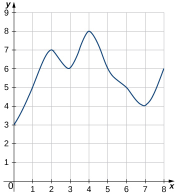
7. The graph of [latex]y={\displaystyle\int }_{0}^{x}f(t)dt,[/latex] where [latex]f[/latex] is a piecewise constant function, is shown here.
   1. Over which intervals is [latex]f[/latex] positive? Over which intervals is it negative? Over which intervals, if any, is it equal to zero?
   2. What are the maximum and minimum values of [latex]f[/latex]?
   3. What is the average value of [latex]f[/latex]?
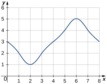
8. The graph of [latex]y={\displaystyle\int }_{0}^{x}\ell (t)dt,[/latex] where ℓ is a piecewise linear function, is shown here.
   1. Over which intervals is ℓ positive? Over which intervals is it negative? Over which, if any, is it zero?
   2. Over which intervals is ℓ increasing? Over which is it decreasing? Over which intervals, if any, is it constant?
   3. What is the average value of ℓ?

In the following exercises (9-21), use a calculator to estimate the area under the curve by computing T₁₀, the average of the left- and right-endpoint Riemann sums using [latex]N=10[/latex] rectangles. Then, using the Fundamental Theorem of Calculus, Part 2, determine the exact area.

9. [latex]y={x}^{3}+6{x}^{2}+x-5[/latex] over [latex]\left[-4,2\right][/latex]
10. [latex]y=\sqrt{x}+{x}^{2}[/latex] over [latex]\left[1,9\right][/latex]
11. [latex]\displaystyle\int \frac{4}{{x}^{2}}dx[/latex] over [latex]\left[1,4\right][/latex]
12. [latex]{\displaystyle\int }_{-2}^{3}({x}^{2}+3x-5)dx[/latex]
13. [latex]{\displaystyle\int }_{2}^{3}({t}^{2}-9)(4-{t}^{2})dt[/latex]
14. [latex]{\displaystyle\int }_{0}^{1}{x}^{99}dx[/latex]
15. [latex]{\displaystyle\int }_{1\text{/}4}^{4}({x}^{2}-\frac{1}{{x}^{2}})dx[/latex]
16. [latex]{\displaystyle\int }_{1}^{4}\frac{1}{2\sqrt{x}}dx[/latex]
17. [latex]{\displaystyle\int }_{1}^{16}\frac{dt}{{t}^{1\text{/}4}}[/latex]
18. [latex]{\displaystyle\int }_{0}^{\pi \text{/}2} \sin \theta d\theta[/latex]
19. [latex]{\displaystyle\int }_{0}^{\pi \text{/}4} \sec \theta \tan {\theta}d\theta[/latex]
20. [latex]{\displaystyle\int }_{\pi \text{/}4}^{\pi \text{/}2}{ \csc }^{2}\theta d\theta[/latex]
21. [latex]{\displaystyle\int }_{-2}^{-1}(\frac{1}{{t}^{2}}-\frac{1}{{t}^{3}})dt[/latex]

In the following exercises (22-23), use the evaluation theorem to express the integral as a function [latex]F(x).[/latex]

22. [latex]{\displaystyle\int }_{1}^{x}{e}^{t}dt[/latex]
23. [latex]{\displaystyle\int }_{\text{−}x}^{x} \sin tdt[/latex]

In the following exercises (24-25), identify the roots of the integrand to remove absolute values, then evaluate using the Fundamental Theorem of Calculus, Part 2.

24. [latex]{\displaystyle\int }_{-2}^{4}|{t}^{2}-2t-3|dt[/latex]
25. [latex]{\displaystyle\int }_{\text{−}\pi \text{/}2}^{\pi \text{/}2}| \sin t|dt[/latex]

For the following exercises (26-29), solve each problem.

26. Suppose the rate of gasoline consumption in the United States can be modeled by a sinusoidal function of the form [latex](11.21- \cos (\frac{\pi t}{6}))×{10}^{9}[/latex] gal/mo.
    1. What is the average monthly consumption, and for which values of [latex]t[/latex] is the rate at time [latex]t[/latex] equal to the average rate?
    2. What is the number of gallons of gasoline consumed in the United States in a year?
    3. Write an integral that expresses the average monthly U.S. gas consumption during the part of the year between the beginning of April [latex](t=3)[/latex] and the end of September [latex](t=9\text{).}[/latex]
27. Explain why, if [latex]f[/latex] is continuous over [latex]\left[a,b\right][/latex] and is not equal to a constant, there is at least one point [latex]M\in \left[a,b\right][/latex] such that [latex]f(M)=\frac{1}{b-a}{\displaystyle\int }_{a}^{b}f(t)dt[/latex] and at least one point [latex]m\in \left[a,b\right][/latex] such that [latex]f(m)<\frac{1}{b-a}{\displaystyle\int }_{a}^{b}f(t)dt.[/latex]
28. A point on an ellipse with major axis length 2[latex]a[/latex] and minor axis length 2[latex]b[/latex] has the coordinates [latex](a \cos \theta ,b \sin \theta ),0\le \theta \le 2\pi .[/latex]
    1. Show that the distance from this point to the focus at [latex](\text{−}c,0)[/latex] is [latex]d(\theta )=a+c \cos \theta ,[/latex] where [latex]c=\sqrt{{a}^{2}-{b}^{2}}.[/latex]
    2. Use these coordinates to show that the average distance [latex]\overline{d}[/latex] from a point on the ellipse to the focus at [latex](\text{−}c,0),[/latex] with respect to angle θ, is [latex]a[/latex].
29. The force of gravitational attraction between the Sun and a planet is [latex]F(\theta )=\frac{GmM}{{r}^{2}(\theta )},[/latex] where [latex]m[/latex] is the mass of the planet, M is the mass of the Sun, G is a universal constant, and [latex]r(\theta )[/latex] is the distance between the Sun and the planet when the planet is at an angle θ with the major axis of its orbit. Assuming that M, [latex]m[/latex], and the ellipse parameters [latex]a[/latex] and [latex]b[/latex] (half-lengths of the major and minor axes) are given, set up—but do not evaluate—an integral that expresses in terms of [latex]G,m,M,a,b[/latex] the average gravitational force between the Sun and the planet.

Integration Formulas and the Net Change Theorem

Use basic integration formulas to compute the following antiderivatives or definite integrals (1-3).

1. [latex]\displaystyle\int (\sqrt{x}-\frac{1}{\sqrt{x}})dx[/latex]
2. [latex]\displaystyle\int \frac{dx}{2x}[/latex]
3. [latex]{\int }_{0}^{\pi }( \sin x- \cos x)dx[/latex]

For the following exercises (4-21), solve each problem.

4. Write an integral that expresses the increase in the perimeter [latex]P(s)[/latex] of a square when its side length [latex]s[/latex] increases from [latex]2[/latex] units to [latex]4[/latex] units and evaluate the integral. 
5. A regular N-gon (an N-sided polygon with sides that have equal length [latex]s[/latex], such as a pentagon or hexagon) has perimeter Ns. Write an integral that expresses the increase in perimeter of a regular N-gon when the length of each side increases from [latex]1[/latex] unit to [latex]2[/latex] units and evaluate the integral.
6. A dodecahedron is a Platonic solid with a surface that consists of [latex]12[/latex] pentagons, each of equal area. By how much does the surface area of a dodecahedron increase as the side length of each pentagon doubles from [latex]1[/latex] unit to [latex]2[/latex] units?
7. Write an integral that quantifies the change in the area of the surface of a cube when its side length doubles from [latex]s[/latex] unit to [latex]2s[/latex] units and evaluate the integral.
8. Write an integral that quantifies the increase in the surface area of a sphere as its radius doubles from R unit to [latex]2[/latex]R units and evaluate the integral.
9. Suppose that a particle moves along a straight line with velocity [latex]v(t)=4-2t,[/latex] where [latex]0\le t\le 2[/latex] (in meters per second). Find the displacement at time [latex]t[/latex] and the total distance traveled up to [latex]t=2.[/latex]
10. Suppose that a particle moves along a straight line with velocity defined by [latex]v(t)=|2t-6|,[/latex] where [latex]0\le t\le 6[/latex] (in meters per second). Find the displacement at time [latex]t[/latex] and the total distance traveled up to [latex]t=6.[/latex]
11. A ball is thrown upward from a height of [latex]1.5[/latex] m at an initial speed of [latex]40[/latex] m/sec. Acceleration resulting from gravity is −[latex]9.8[/latex] m/sec². Neglecting air resistance, solve for the velocity [latex]v(t)[/latex] and the height [latex]h(t)[/latex] of the ball [latex]t[/latex] seconds after it is thrown and before it returns to the ground.
12. The area [latex]A(t)[/latex] of a circular shape is growing at a constant rate. If the area increases from [latex]4[/latex]π units to [latex]9[/latex]π units between times [latex]t=2[/latex] and [latex]t=3,[/latex] find the net change in the radius during that time.
13. Water flows into a conical tank with cross-sectional area πx² at height [latex]x[/latex] and volume [latex]\frac{\pi {x}^{3}}{3}[/latex] up to height [latex]x[/latex]. If water flows into the tank at a rate of [latex]1[/latex] m³/min, find the height of water in the tank after [latex]5[/latex] min. Find the change in height between [latex]5[/latex] min and [latex]10[/latex] min.
14. The following table lists the electrical power in gigawatts—the rate at which energy is consumed—used in a certain city for different hours of the day, in a typical 24-hour period, with hour [latex]1[/latex] corresponding to midnight to 1 a.m.
    

    Hour	Power	Hour	Power
    [latex]1[/latex]	[latex]28[/latex]	[latex]13[/latex]	[latex]48[/latex]
    [latex]2[/latex]	[latex]25[/latex]	[latex]14[/latex]	[latex]49[/latex]
    [latex]3[/latex]	[latex]24[/latex]	[latex]15[/latex]	[latex]49[/latex]
    [latex]4[/latex]	[latex]23[/latex]	[latex]16[/latex]	[latex]50[/latex]
    [latex]5[/latex]	[latex]24[/latex]	[latex]17[/latex]	[latex]50[/latex]
    [latex]6[/latex]	[latex]27[/latex]	[latex]18[/latex]	[latex]50[/latex]
    [latex]7[/latex]	[latex]29[/latex]	[latex]19[/latex]	[latex]46[/latex]
    [latex]8[/latex]	[latex]32[/latex]	[latex]20[/latex]	[latex]43[/latex]
    [latex]9[/latex]	[latex]34[/latex]	[latex]21[/latex]	[latex]42[/latex]
    [latex]10[/latex]	[latex]39[/latex]	[latex]22[/latex]	[latex]40[/latex]
    [latex]11[/latex]	[latex]42[/latex]	[latex]23[/latex]	[latex]37[/latex]
    [latex]12[/latex]	[latex]46[/latex]	[latex]24[/latex]	[latex]34[/latex]

    Find the total amount of power in gigawatt-hours (gW-h) consumed by the city in a typical 24-hour period.

15. The data in the following table are used to estimate the average power output produced by Peter Sagan for each of the last [latex]18[/latex] sec of Stage 1 of the 2012 Tour de France.
    

    Average Power OutputSource: sportsexercisengineering.com

    Second	Watts	Second	Watts
    [latex]1[/latex]	[latex]600[/latex]	[latex]10[/latex]	[latex]1200[/latex]
    [latex]2[/latex]	[latex]500[/latex]	[latex]11[/latex]	[latex]1170[/latex]
    [latex]3[/latex]	[latex]575[/latex]	[latex]12[/latex]	[latex]1125[/latex]
    [latex]4[/latex]	[latex]1050[/latex]	[latex]13[/latex]	[latex]1100[/latex]
    [latex]5[/latex]	[latex]925[/latex]	[latex]14[/latex]	[latex]1075[/latex]
    [latex]6[/latex]	[latex]950[/latex]	[latex]15[/latex]	[latex]1000[/latex]
    [latex]7[/latex]	[latex]1050[/latex]	[latex]16[/latex]	[latex]950[/latex]
    [latex]8[/latex]	[latex]950[/latex]	[latex]17[/latex]	[latex]900[/latex]
    [latex]9[/latex]	[latex]1100[/latex]	[latex]18[/latex]	[latex]780[/latex]

    Estimate the net energy used in kilojoules (kJ), noting that [latex]1[/latex]W [latex]= 1[/latex] J/s, and the average power output by Sagan during this time interval.

16. The distribution of incomes as of 2012 in the United States in [latex]$5000[/latex] increments is given in the following table. The [latex]k[/latex]th row denotes the percentage of households with incomes between [latex]$5000xk[/latex] and [latex]5000xk+4999.[/latex] The row [latex]k=40[/latex] contains all households with income between [latex]$200,000[/latex] and [latex]$250,000[/latex] and [latex]k=41[/latex] accounts for all households with income exceeding [latex]$250,000[/latex].
    

    Income DistributionsSource: http://www.census.gov/prod/2013pubs/p60-245.pdf

    [latex]0[/latex]	[latex]3.5[/latex]	[latex]21[/latex]	[latex]1.5[/latex]
    [latex]1[/latex]	[latex]4.1[/latex]	[latex]22[/latex]	[latex]1.4[/latex]
    [latex]2[/latex]	[latex]5.9[/latex]	[latex]23[/latex]	[latex]1.3[/latex]
    [latex]3[/latex]	[latex]5.7[/latex]	[latex]24[/latex]	[latex]1.3[/latex]
    [latex]4[/latex]	[latex]5.9[/latex]	[latex]25[/latex]	[latex]1.1[/latex]
    [latex]5[/latex]	[latex]5.4[/latex]	[latex]26[/latex]	[latex]1.0[/latex]
    [latex]6[/latex]	[latex]5.5[/latex]	[latex]27[/latex]	[latex]0.75[/latex]
    [latex]7[/latex]	[latex]5.1[/latex]	[latex]28[/latex]	[latex]0.8[/latex]
    [latex]8[/latex]	[latex]4.8[/latex]	[latex]29[/latex]	[latex]1.0[/latex]
    [latex]9[/latex]	[latex]4.1[/latex]	[latex]30[/latex]	[latex]0.6[/latex]
    [latex]10[/latex]	[latex]4.3[/latex]	[latex]31[/latex]	[latex]0.6[/latex]
    [latex]11[/latex]	[latex]3.5[/latex]	[latex]32[/latex]	[latex]0.5[/latex]
    [latex]12[/latex]	[latex]3.7[/latex]	[latex]33[/latex]	[latex]0.5[/latex]
    [latex]13[/latex]	[latex]3.2[/latex]	[latex]34[/latex]	[latex]0.4[/latex]
    [latex]14[/latex]	[latex]3.0[/latex]	[latex]35[/latex]	[latex]0.3[/latex]
    [latex]15[/latex]	[latex]2.8[/latex]	[latex]36[/latex]	[latex]0.3[/latex]
    [latex]16[/latex]	[latex]2.5[/latex]	[latex]37[/latex]	[latex]0.3[/latex]
    [latex]17[/latex]	[latex]2.2[/latex]	[latex]38[/latex]	[latex]0.2[/latex]
    [latex]18[/latex]	[latex]2.2[/latex]	[latex]39[/latex]	[latex]1.8[/latex]
    [latex]19[/latex]	[latex]1.8[/latex]	[latex]40[/latex]	[latex]2.3[/latex]
    [latex]20[/latex]	[latex]2.1[/latex]	[latex]41[/latex]

    1. Estimate the percentage of U.S. households in 2012 with incomes less than [latex]$55,000[/latex].
    2. What percentage of households had incomes exceeding [latex]$85,000[/latex]?
    3. Plot the data and try to fit its shape to that of a graph of the form [latex]a(x+c){e}^{\text{−}b(x+e)}[/latex] for suitable [latex]a,b,c.[/latex]
17. For a given motor vehicle, the maximum achievable deceleration from braking is approximately [latex]7[/latex] m/sec² on dry concrete. On wet asphalt, it is approximately [latex]2.5[/latex] m/sec². Given that 1 mph corresponds to [latex]0.447[/latex] m/sec, find the total distance that a car travels in meters on dry concrete after the brakes are applied until it comes to a complete stop if the initial velocity is [latex]67[/latex] mph ([latex]30[/latex] m/sec) or if the initial braking velocity is [latex]56[/latex] mph ([latex]25[/latex] m/sec). Find the corresponding distances if the surface is slippery wet asphalt.
18. Sandra is a [latex]25[/latex]-year old woman who weighs [latex]120[/latex] lb. She burns [latex]300-50t[/latex] cal/hr while walking on her treadmill. Her caloric intake from drinking Gatorade is [latex]100t[/latex] calories during the [latex]t[/latex]th hour. What is her net decrease in calories after walking for [latex]3[/latex] hours?
19. Although some engines are more efficient at given a horsepower than others, on average, fuel efficiency decreases with horsepower at a rate of [latex]1\text{/}25[/latex] mpg/horsepower. If a typical [latex]50[/latex]-horsepower engine has an average fuel efficiency of [latex]32[/latex] mpg, what is the average fuel efficiency of an engine with the following horsepower: [latex]150[/latex], [latex]300[/latex], [latex]450[/latex]?
20. The following table provides hypothetical data regarding the level of service for a certain highway.
    

    Highway Speed Range (mph)	Vehicles per Hour per Lane	Density Range (vehicles/mi)
    [latex]> 60[/latex]	[latex]< 600[/latex]	[latex]< 10[/latex]
    [latex]60–57[/latex]	[latex]600–1000[/latex]	[latex]10–20[/latex]
    [latex]57–54[/latex]	[latex]1000–1500[/latex]	[latex]20–30[/latex]
    [latex]54–46[/latex]	[latex]1500–1900[/latex]	[latex]30–45[/latex]
    [latex]46–30[/latex]	[latex]1900–2100[/latex]	[latex]45–70[/latex]
    [latex]<30[/latex]	Unstable	[latex]70–200[/latex]

    1. Plot vehicles per hour per lane on the [latex]x[/latex]-axis and highway speed on the [latex]y[/latex]-axis.
    2. Compute the average decrease in speed (in miles per hour) per unit increase in congestion (vehicles per hour per lane) as the latter increases from [latex]600[/latex] to [latex]1000[/latex], from [latex]1000[/latex] to [latex]1500[/latex], and from [latex]1500[/latex] to [latex]2100[/latex]. Does the decrease in miles per hour depend linearly on the increase in vehicles per hour per lane?
    3. Plot minutes per mile ([latex]60[/latex] times the reciprocal of miles per hour) as a function of vehicles per hour per lane. Is this function linear?
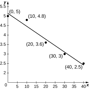
21. An athlete runs by a motion detector, which records her speed, as displayed in the following table. The best linear fit to this data, [latex]\ell (t)=-0.068t+5.14\text{,}[/latex] is shown in the accompanying graph. Use the average value of [latex]\ell (t)[/latex] between [latex]t=0[/latex] and [latex]t=40[/latex] to estimate the runner’s average speed.
    

    Minutes	Speed (m/sec)
    [latex]0[/latex]	[latex]5[/latex]
    [latex]10[/latex]	[latex]4.8[/latex]
    [latex]20[/latex]	[latex]3.6[/latex]
    [latex]30[/latex]	[latex]3.0[/latex]
    [latex]40[/latex]	[latex]2.5[/latex]