- Identify hyperbolic functions their graphs, and understand their fundamental identities
Hyperbolic Functions
Hyperbolic functions are defined in terms of certain combinations of [latex]e^x[/latex] and [latex]e^{−x}[/latex]. These functions arise naturally in various engineering and physics applications, including the study of water waves and vibrations of elastic membranes.
Another common use for a hyperbolic function is the representation of a hanging chain or cable, also known as a catenary. If we introduce a coordinate system so that the low point of the chain lies along the [latex]y[/latex]-axis, we can describe the height of the chain in terms of a hyperbolic function.

Using the definition of [latex]\cosh(x)[/latex] and principles of physics, it can be shown that the height of a hanging chain can be described by the function [latex]h(x)=a \cosh(x/a)+c[/latex] for certain constants [latex]a[/latex] and [latex]c[/latex].
hyperbolic functions
Hyperbolic cosine
Hyperbolic sine
Hyperbolic tangent
Hyperbolic cosecant
Hyperbolic secant
Hyperbolic cotangent
The name cosh rhymes with “gosh,” whereas the name sinh is pronounced “cinch.” Tanh, sech, csch, and coth are pronounced “tanch,” “seech,” “coseech,” and “cotanch,” respectively.
But why are these functions called hyperbolic functions?
To answer this question, consider the quantity [latex]\cosh^2 t-\sinh^2 t[/latex]. Using the definition of [latex]\cosh[/latex] and [latex]\sinh[/latex], we see that
This identity is the analog of the trigonometric identity [latex]\cos^2 t+\sin^2 t=1[/latex]. Here, given a value [latex]t[/latex], the point [latex](x,y)=(\cosh t,\sinh t)[/latex] lies on the unit hyperbola [latex]x^2-y^2=1[/latex] (Figure 7).
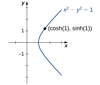
If you think hyperbolic functions look a lot like trigonometric ones, you’re not wrong! They share similar properties because they’re both connected to the concept of the exponential function [latex]e^x[/latex]. Remember, while trigonometric functions relate to the unit circle, hyperbolic functions are associated with the unit hyperbola.
Graphs of Hyperbolic Functions
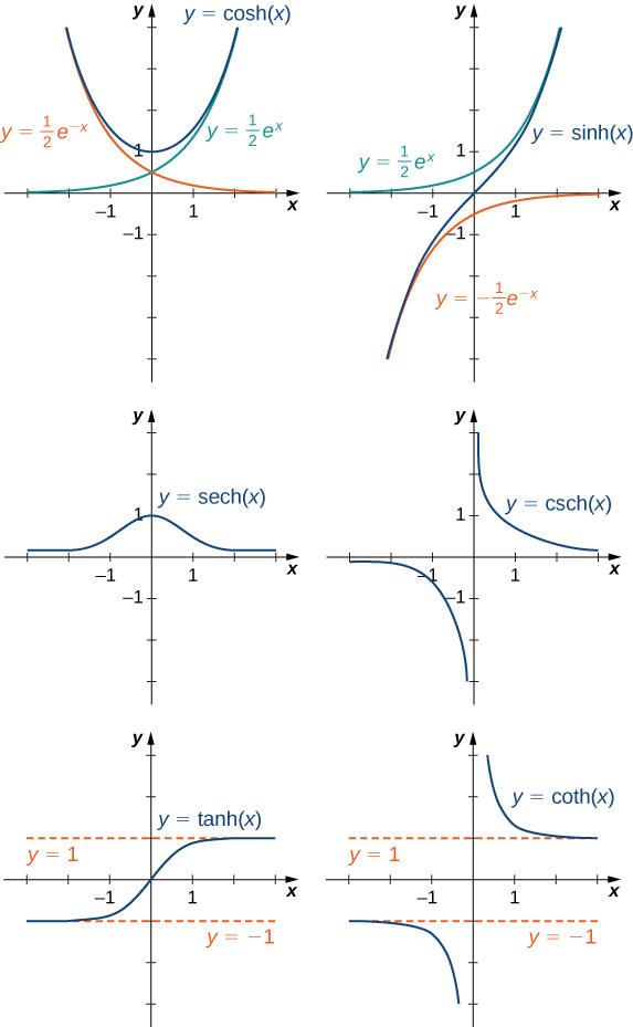
The graphs of [latex]\cosh x[/latex] and [latex]\sinh x[/latex], can be derived by observing how they relate to exponential functions.
As [latex]x[/latex] approaches towards infinity, both functions approach [latex]\frac{1}{2}e^x[/latex] because the term [latex]e^{−x}[/latex] becomes negligible.
In contrast, as [latex]x[/latex] moves towards negative infinity, [latex]\cosh x[/latex] mirrors [latex]\frac{1}{2}e^{−x}[/latex], while [latex]\sinh x[/latex] mirrors [latex]-\frac{1}{2}e^{−x}[/latex].
Therefore, the graphs [latex]\frac{1}{2}e^x, \, \frac{1}{2}e^{−x}[/latex], and [latex]−\frac{1}{2}e^{−x}[/latex] provide a roadmap for sketching the graphs.
When graphing [latex]\tanh x[/latex], we note that its value starts at [latex]0[/latex] when [latex]x[/latex] is [latex]0[/latex] and then ascends towards [latex]1[/latex] or descends towards [latex]-1[/latex] as [latex]x[/latex] goes to positive or negative infinity, respectively.
The graphs of the other three hyperbolic functions can be sketched using the graphs of [latex]\cosh x, \, \sinh x[/latex], and [latex]\tanh x[/latex] (Figure 8).
Identities Involving Hyperbolic Functions
Just as trigonometric functions have identities that allow for the simplification and transformation of expressions, hyperbolic functions also possess their own set of identities.
hyperbolic function identities
- [latex]\cosh(−x)=\cosh x[/latex]
- [latex]\sinh(−x)=−\sinh x[/latex]
Hyperbolic Pythagorean Identities:
- [latex]\cosh^2 x-\sinh^2 x=1[/latex]
Hyperbolic Squared Identities:
- [latex]1-\tanh^2 x=\text{sech}^2 x[/latex]
- [latex]\coth^2 x-1=\text{csch}^2 x[/latex]
Hyperbolic Addition Formulas:
- [latex]\sinh(x \pm y)=\sinh x \cosh y \pm \cosh x \sinh y[/latex]
- [latex]\cosh (x \pm y)=\cosh x \cosh y \pm \sinh x \sinh y[/latex]
Exponential Definitions of Hyperbolic Functions
- [latex]\cosh x+\sinh x=e^x[/latex]
- [latex]\cosh x-\sinh x=e^{−x}[/latex]
- Simplify [latex]\sinh(5 \ln x)[/latex].
- If [latex]\sinh x=\frac{3}{4}[/latex], find the values of the remaining five hyperbolic functions.