Defining the Number [latex]e[/latex]
Now that we have the natural logarithm defined, we can use that function to define the number [latex]e.[/latex]
the number [latex]e[/latex]
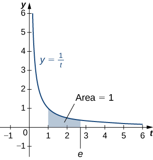
The number [latex]e[/latex] is defined to be the real number such that
To put it another way, the area under the curve [latex]y=\frac{1}{t}[/latex] between [latex]t=1[/latex] and [latex]t=e[/latex] is [latex]1[/latex] (Figure 3).
The proof that such a number exists and is unique is left to you. (Hint: Use the Intermediate Value Theorem to prove existence and the fact that [latex]\text{ln}x[/latex] is increasing to prove uniqueness.)
The number [latex]e[/latex] can be shown to be irrational, although we won’t do so here. Its approximate value is given by
The Exponential Function
We now turn our attention to the function [latex]{e}^{x}.[/latex] Note that the natural logarithm is one-to-one and therefore has an inverse function. For now, we denote this inverse function by [latex]\text{exp }x.[/latex] Then,
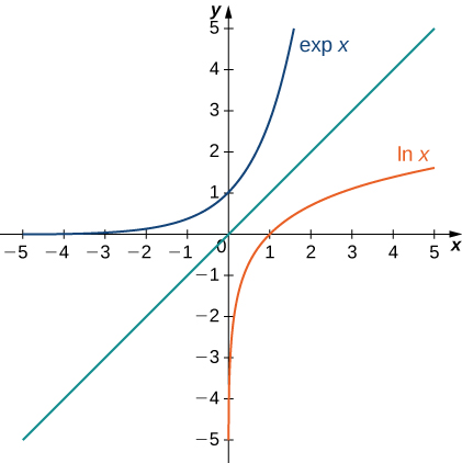
The following figure shows the graphs of [latex]\text{exp }x[/latex] and [latex]\text{ln }x.[/latex]
We hypothesize that [latex]\text{exp }x={e}^{x}.[/latex]
For rational values of [latex]x,[/latex] this is easy to show. If [latex]x[/latex] is rational, then we have [latex]\text{ln }({e}^{x})=x\text{ln }e=x.[/latex] Thus, when [latex]x[/latex] is rational, [latex]{e}^{x}=\text{exp }x.[/latex]
For irrational values of [latex]x,[/latex] we simply define [latex]{e}^{x}[/latex] as the inverse function of [latex]\text{ln }x.[/latex]
defining the exponential function
For any real number [latex]x,[/latex] define [latex]y={e}^{x}[/latex] to be the number for which
Then we have [latex]{e}^{x}=\text{exp}(x)[/latex] for all [latex]x,[/latex] and thus
for all [latex]x.[/latex]
Properties of the Exponential Function
Since the exponential function was defined in terms of an inverse function, and not in terms of a power of [latex]e,[/latex] we must verify that the usual laws of exponents hold for the function [latex]{e}^{x}.[/latex]
properties of the exponential function
If [latex]p[/latex] and [latex]q[/latex] are any real numbers and [latex]r[/latex] is a rational number, then
- [latex]{e}^{p}{e}^{q}={e}^{p+q}[/latex]
- [latex]\frac{{e}^{p}}{{e}^{q}}={e}^{p-q}[/latex]
- [latex]{({e}^{p})}^{r}={e}^{pr}[/latex]
Proof
Note that if [latex]p[/latex] and [latex]q[/latex] are rational, the properties hold. However, if [latex]p[/latex] or [latex]q[/latex] are irrational, we must apply the inverse function definition of [latex]{e}^{x}[/latex] and verify the properties. Only the first property is verified here; the other two are left to you. We have
Since [latex]\text{ln}x[/latex] is one-to-one, then
[latex]_\blacksquare[/latex]
As with part iv. of the logarithm properties, we can extend property iii. to irrational values of [latex]r,[/latex] and we do so by the end of the section.
We also want to verify the differentiation formula for the function [latex]y={e}^{x}.[/latex]
To do this, we need to use implicit differentiation. Let [latex]y={e}^{x}.[/latex] Then,
Thus, we see
as desired, which leads immediately to the integration formula
We apply these formulas in the following examples.
Evaluate the following derivatives:
- [latex]\frac{d}{dt}{e}^{3t}{e}^{{t}^{2}}[/latex]
- [latex]\frac{d}{dx}{e}^{3{x}^{2}}[/latex]
Evaluate the following integral: [latex]\displaystyle\int \frac{4}{{e}^{3x}}dx.[/latex]