Exponential Decay Model
Exponential functions can also be used to model populations that shrink (from disease, for example), or chemical compounds that break down over time. We say that such systems exhibit exponential decay, rather than exponential growth. The model is nearly the same, except there is a negative sign in the exponent. Thus, for some positive constant [latex]k,[/latex] we have
[latex]y={y}_{0}{e}^{\text{−}kt}.[/latex]
As with exponential growth, there is a differential equation associated with exponential decay. We have
exponential decay model
Systems that exhibit exponential decay behave according to the model
where [latex]{y}_{0}[/latex] represents the initial state of the system and [latex]k>0[/latex] is a constant, called the decay constant.
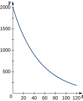
The following figure shows a graph of a representative exponential decay function.
Let’s look at a physical application of exponential decay.
Newton’s Law of Cooling
Newton’s law of cooling says that an object cools at a rate proportional to the difference between the temperature of the object and the temperature of the surroundings.
In other words, if [latex]T[/latex] represents the temperature of the object and [latex]{T}_{a}[/latex] represents the ambient temperature in a room, then
Note that this is not quite the right model for exponential decay. We want the derivative to be proportional to the function, and this expression has the additional [latex]{T}_{a}[/latex] term. Fortunately, we can make a change of variables that resolves this issue.
Let [latex]y(t)=T(t)-{T}_{a}.[/latex] Then [latex]{y}^{\prime }(t)={T}^{\prime }(t)-0={T}^{\prime }(t),[/latex] and our equation becomes
From our previous work, we know this relationship between [latex]y[/latex] and its derivative leads to exponential decay. Thus,
and we see that
where [latex]{T}_{0}[/latex] represents the initial temperature.
Let’s apply this formula in the following example.
According to experienced baristas, the optimal temperature to serve coffee is between [latex]155\text{°}\text{F}[/latex] and [latex]175\text{°}\text{F}.[/latex] Suppose coffee is poured at a temperature of [latex]200\text{°}\text{F},[/latex] and after 2 minutes in a [latex]70\text{°}\text{F}[/latex] room it has cooled to [latex]180\text{°}\text{F}.[/latex] When is the coffee first cool enough to serve? When is the coffee too cold to serve? Round answers to the nearest half minute.
Half-Life and Radioactive Decay
Just as systems exhibiting exponential growth have a constant doubling time, systems exhibiting exponential decay have a constant half-life.
To calculate the half-life, we want to know when the quantity reaches half its original size. Therefore, we have
Note: This is the same expression we came up with for doubling time.
half-life
If a quantity decays exponentially, the half-life is the amount of time it takes the quantity to be reduced by half. It is given by
One of the most common applications of an exponential decay model is carbon dating. [latex]\text{Carbon-}14[/latex] decays (emits a radioactive particle) at a regular and consistent exponential rate. Therefore, if we know how much carbon was originally present in an object and how much carbon remains, we can determine the age of the object.
The half-life of [latex]\text{carbon-}14[/latex] is approximately [latex]5730[/latex] years—meaning, after that many years, half the material has converted from the original [latex]\text{carbon-}14[/latex] to the new nonradioactive [latex]\text{nitrogen-}14.[/latex]
Another example of radioactive decay is uranium-238, which decays into lead-206 over a much longer period, with a half-life of about [latex]4.5[/latex] billion years. This property is often used to date rocks and fossils, providing important insights into the history of the Earth and its geological events.
If we have [latex]100[/latex] g [latex]\text{carbon-}14[/latex] today, how much is left in [latex]50[/latex] years?
If an artifact that originally contained [latex]100[/latex] g of carbon now contains [latex]10[/latex] g of carbon, how old is it? Round the answer to the nearest hundred years.