- Apply the exponential growth formula to real-world cases like increasing populations or investments
- Describe how long it takes for quantities to double or reduce by half
- Implement the exponential decay formula for scenarios like radioactive substances decaying or objects cooling down
Exponential Growth Model
Many systems exhibit exponential growth. These systems follow a model of the form [latex]y={y}_{0}{e}^{kt},[/latex] where [latex]{y}_{0}[/latex] represents the initial state of the system and [latex]k[/latex] is a positive constant, called the growth constant.
Notice that in an exponential growth model, we have
That is, the rate of growth is proportional to the current function value. This is a key feature of exponential growth.
exponential growth model
Systems that exhibit exponential growth increase according to the mathematical model
where [latex]{y}_{0}[/latex] represents the initial state of the system and [latex]k>0[/latex] is a constant, called the growth constant.
Population Growth
Population growth is a common example of exponential growth.
Consider a population of bacteria, for instance. It seems plausible that the rate of population growth would be proportional to the size of the population. After all, the more bacteria there are to reproduce, the faster the population grows.
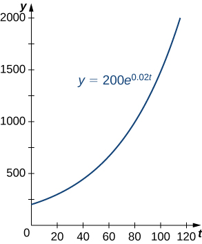
Figure 1 and the table below represent the growth of a population of bacteria with an initial population of [latex]200[/latex] bacteria and a growth constant of [latex]0.02[/latex]. Notice that after only [latex]2[/latex] hours [latex](120[/latex] minutes), the population is [latex]10[/latex] times its original size!
| Time (min) | Population Size (no. of bacteria) |
|---|---|
| 10 | 244 |
| 20 | 298 |
| 30 | 364 |
| 40 | 445 |
| 50 | 544 |
| 60 | 664 |
| 70 | 811 |
| 80 | 991 |
| 90 | 1210 |
| 100 | 1478 |
| 110 | 1805 |
| 120 | 2205 |
Note that we are using a continuous function to model what is inherently discrete behavior. At any given time, the real-world population contains a whole number of bacteria, although the model takes on noninteger values. When using exponential growth models, we must always be careful to interpret the function values in the context of the phenomenon we are modeling.
Consider the population of bacteria described earlier. This population grows according to the function [latex]f(t)=200{e}^{0.02t},[/latex] where [latex]t[/latex] is measured in minutes. How many bacteria are present in the population after 5 hours [latex](300[/latex] minutes)? When does the population reach 100,000 bacteria?
Let’s now turn our attention to a financial application: compound interest.
Compound Interest
Interest that is not compounded is called simple interest. Simple interest is paid once, at the end of the specified time period (usually 1 year).
If we put [latex]$1000[/latex] in a savings account earning [latex]2\%[/latex] simple interest per year, then at the end of the year we have,
Compound interest is paid multiple times per year, depending on the compounding period.
If a bank compounds the interest every [latex]6[/latex] months, it credits half of the year’s interest to the account after [latex]6[/latex] months.
During the second half of the year, the account earns interest not only on the initial [latex]$1000,[/latex] but also on the interest earned during the first half of the year. Mathematically speaking, at the end of the year, we have
Similarly, if the interest is compounded every [latex]4[/latex] months, we have
and if the interest is compounded daily [latex](365[/latex] times per year), we have [latex]$1020.20.[/latex]
If we extend this concept, so that the interest is compounded continuously, after [latex]t[/latex] years we have
Now let’s manipulate this expression so that we have an exponential growth function. Recall that the number [latex]e[/latex] can be expressed as a limit:
Based on this, we want the expression inside the parentheses to have the form [latex](1+1\text{/}m).[/latex] Let [latex]n=0.02m.[/latex] Note that as [latex]n\to \infty ,[/latex] [latex]m\to \infty[/latex] as well. Then we get
We recognize the limit inside the brackets as the number [latex]e.[/latex] So, the balance in our bank account after [latex]t[/latex] years is given by [latex]1000{e}^{0.02t}.[/latex]
Generalizing this concept, we see that if a bank account with an initial balance of [latex]$P[/latex] earns interest at a rate of [latex]r\text{%},[/latex] compounded continuously, then the balance of the account after [latex]t[/latex] years is
A 25-year-old student is offered an opportunity to invest some money in a retirement account that pays [latex]5\%[/latex] annual interest compounded continuously. How much does the student need to invest today to have [latex]$1[/latex] million when she retires at age [latex]65?[/latex]
What if she could earn [latex]6\%[/latex] annual interest compounded continuously instead?
Doubling Time
If a quantity grows exponentially, the time it takes for the quantity to double remains constant. In other words, it takes the same amount of time for a population of bacteria to grow from [latex]100[/latex] to [latex]200[/latex] bacteria as it does to grow from [latex]10,000[/latex] to [latex]20,000[/latex] bacteria. This time is called the doubling time.
To calculate the doubling time, we want to know when the quantity reaches twice its original size. So we have
doubling time
If a quantity grows exponentially, the doubling time is the amount of time it takes the quantity to double. It is given by
Assume a population of fish grows exponentially. A pond is stocked initially with [latex]500[/latex] fish. After [latex]6[/latex] months, there are [latex]1000[/latex] fish in the pond. The owner will allow his friends and neighbors to fish on his pond after the fish population reaches [latex]10,000[/latex]. When will the owner’s friends be allowed to fish?