Exponential and Logarithmic Functions: Learn It 1

Lumen Learning

Exponential and Logarithmic Functions: Learn It 1

Work with exponential functions to find their values
Recognize logarithmic functions, explore their relationship with exponential functions, and change their bases
Identify hyperbolic functions their graphs, and understand their fundamental identities

Exponential Functions

Exponential functions arise in many applications. One common example is population growth.

If a population starts with $P_0$ individuals and then grows at an annual rate of $2\%$ , its population after $1$ year is

P (1) = P_{0} + 0.02 P_{0} = P_{0} (1 + 0.02) = P_{0} (1.02)

$P(1)=P_0+0.02P_0=P_0(1+0.02)=P_0(1.02)$

Its population after $2$ years is

P (2) = P (1) + 0.02 P (1) = P (1) (1.02) = P_{0} (1.02)^{2}

$P(2)=P(1)+0.02P(1)=P(1)(1.02)=P_0(1.02)^2$

In general, its population after $t$ years is

P (t) = P_{0} (1.02)^{t}

$P(t)=P_0(1.02)^t$ ,

which is an exponential function.

More generally, any function of the form $f(x)=b^x$ , where $b>0, \, b \ne 1$ , is an exponential function with base $b$ and exponent $x$ . Exponential functions have constant bases and variable exponents.

exponential function

For any real number $x$ , an exponential function is a function with the form

$f(x)=ab^x$

where,

$a$ is a non-zero real number called the initial value and
$b$ is any positive real number ( $b>0$ ) such that $b≠1$ .

Why do we limit the base $b$ to positive values?

To ensure that the outputs will be real numbers. Observe what happens if the base is not positive:

Let $b=−9$ and $x=\frac{1}{2}$ . Then $f(x)=f(\frac{1}{2})=(−9)^\frac{1}{2}=\sqrt{−9}$ , which is not a real number.

Why do we limit the base to positive values other than $1$ ?

Because base $1$ results in the constant function. Observe what happens if the base is $1$ :

Let $b=1$ . Then $f(x)=1^x=1$ for any value of $x$ .

Note that a function of the form $f(x)=x^b$ for some constant $b$ is not an exponential function but a power function.

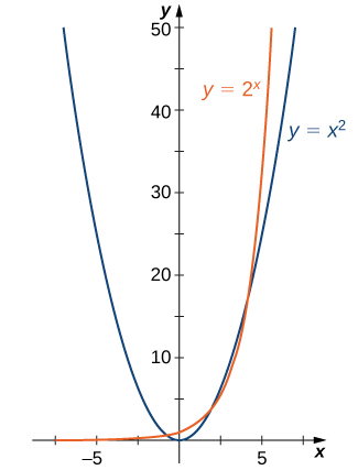
To see the difference between an exponential function and a power function, we can compare the functions $y=x^2$ and $y=2^x$ .

In the table below, we see that both $2^x$ and $x^2$ approach infinity as $x \to \infty$ . Eventually, however, $2^x$ becomes larger than $x^2$ and grows more rapidly as $x \to \infty$ . In the opposite direction, as $x \to −\infty, \, x^2 \to \infty$ , whereas $2^x \to 0$ . The line $y=0$ is a horizontal asymptote for $y=2^x$ .

Values of $x^2$ and $2^x$
$\mathbf{x}$	$\mathbf{x^2}$	$\mathbf{2^x}$
$-3$	$9$	$1/8$
$-2$	$4$	$1/4$
$-1$	$1$	$1/2$
$0$	$0$	$1$
$1$	$1$	$2$
$2$	$4$	$4$
$3$	$9$	$8$
$4$	$16$	$16$
$5$	$25$	$32$
$6$	$36$	$64$

An image of a graph. The x axis runs from -10 to 10 and the y axis runs from 0 to 50. The graph is of two functions. The first function is “y = x squared”, which is a parabola. The function decreases until it hits the origin and then begins increasing. The second function is “y = 2 to the power of x”, which starts slightly above the x axis, and begins increasing very rapidly, more rapidly than the first function. — Figure 1. Both $2^x$ and $x^2$ approach infinity as $x \to \infty$ , but $2^x$ grows more rapidly than $x^2$ . As $x \to −\infty, \, x^2 \to \infty$ , whereas $2^x \to 0$ .

Arrow Notation
Symbol	Meaning
$x\to \infty$	$x$ approaches infinity ( $x$ increases without bound)
$x\to -\infty$	$x$ approaches negative infinity ( $x$ decreases without bound)
$f\left(x\right)\to \infty$	the output approaches infinity (the output increases without bound)
$f\left(x\right)\to -\infty$	the output approaches negative infinity (the output decreases without bound)
$f\left(x\right)\to a$	the output approaches $a$