The Disk Method

When we use the slicing method with solids of revolution, it is often called the disk method because, for solids of revolution, the slices used to over approximate the volume of the solid are disks.

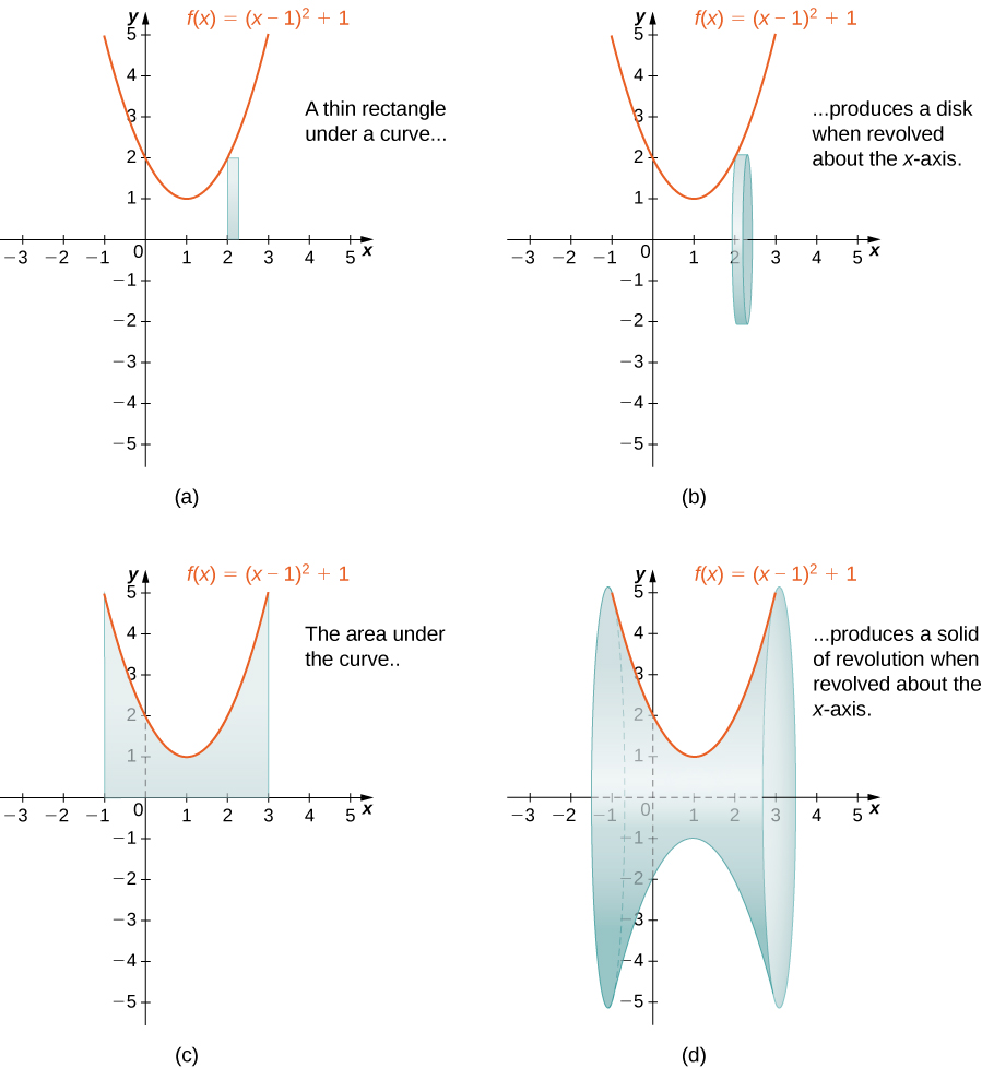
To see this, consider the solid of revolution generated by revolving the region between the graph of the function [latex]f(x)={(x-1)}^{2}+1[/latex] and the [latex]x\text{-axis}[/latex] over the interval [latex]\left[-1,3\right][/latex] around the [latex]x\text{-axis}\text{.}[/latex] 

We already used the formal Riemann sum development of the volume formula when we developed the slicing method. We know that

The only difference with the disk method is that we know the formula for the cross-sectional area ahead of time; it is the area of a circle. 

Returning to our example, the volume is given by:

Use the disk method to find the volume of the solid of revolution generated by rotating the region between the graph of [latex]f(x)=\sqrt{x}[/latex] and the [latex]x\text{-axis}[/latex] over the interval [latex]\left[1,4\right][/latex] around the [latex]x\text{-axis}\text{.}[/latex]

Show Solution

The graphs of the function and the solid of revolution are shown in the following figure.

We have

[latex]\begin{array}{cc}\hfill V& ={\displaystyle\int }_{a}^{b}\pi {\left[f(x)\right]}^{2}dx\hfill \\ & ={\displaystyle\int }_{1}^{4}\pi {\left[\sqrt{x}\right]}^{2}dx=\pi {\displaystyle\int }_{1}^{4}xdx\hfill \\ & ={\frac{\pi }{2}{x}^{2}|}_{1}^{4}=\frac{15\pi }{2}.\hfill \end{array}[/latex]

The volume is [latex]\frac{(15\pi )}{2}[/latex] units³.

So far, our examples have all concerned regions revolved around the [latex]x\text{-axis,}[/latex] but we can generate a solid of revolution by revolving a plane region around any horizontal or vertical line.

In the next example, we look at a solid of revolution that has been generated by revolving a region around the [latex]y\text{-axis}\text{.}[/latex] The mechanics of the disk method are nearly the same as when the [latex]x\text{-axis}[/latex] is the axis of revolution, but we express the function in terms of [latex]y[/latex] and we integrate with respect to [latex]y[/latex] as well. 

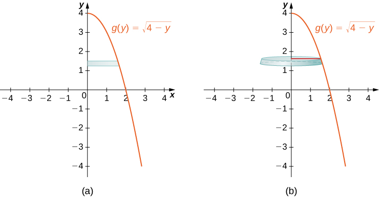
Let [latex]R[/latex] be the region bounded by the graph of [latex]g(y)=\sqrt{4-y}[/latex] and the [latex]y\text{-axis}[/latex] over the [latex]y\text{-axis}[/latex] interval [latex]\left[0,4\right].[/latex] Use the disk method to find the volume of the solid of revolution generated by rotating [latex]R[/latex] around the [latex]y\text{-axis}\text{.}[/latex]

Show Solution

Figure 11 shows the function and a representative disk that can be used to estimate the volume. Notice that since we are revolving the function around the [latex]y\text{-axis,}[/latex] the disks are horizontal, rather than vertical.

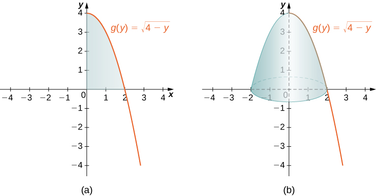
The region to be revolved and the full solid of revolution are depicted in the following figure.

To find the volume, we integrate with respect to [latex]y.[/latex] We obtain

[latex]\begin{array}{cc}\hfill V& ={\displaystyle\int }_{c}^{d}\pi {\left[g(y)\right]}^{2}dy\hfill \\ & ={\displaystyle\int }_{0}^{4}\pi {\left[\sqrt{4-y}\right]}^{2}dy=\pi {\displaystyle\int }_{0}^{4}(4-y)dy\hfill \\ & ={\pi \left[4y-\frac{{y}^{2}}{2}\right]|}_{0}^{4}=8\pi .\hfill \end{array}[/latex]

 

The volume is [latex]8\pi[/latex] units³.