Derivatives of Exponential and Logarithmic Functions: Learn It 1

Lumen Learning

Derivatives of Exponential and Logarithmic Functions: Learn It 1

Determine the derivatives of exponential and logarithmic functions
Apply logarithmic differentiation to find derivatives

Exponential and logarithmic functions are crucial in modeling growth processes, such as population dynamics and radioactive decay. These functions also simplify complex mathematical expressions. In this section, we delve deeper into their derivatives, highlighting the uniqueness of these functions, particularly through the properties of the natural exponential function, $e^x$ .

Derivative of the Exponential Function

The differentiation of exponential functions $B(x)=b^x$ where $b>0$ , begins with recognizing that these functions are defined for all real numbers and are continuous. This universality stems from the properties defined for exponentiation over rational and irrational numbers alike.

Historically, exponentiation for integers was defined straightforwardly—for example, $b^n$ where $n$ is an integer. For non-integer exponents, $b^r$ (where $r$ is any real number), we interpret this through a limiting process. Specifically, $b^r$ is understood as the limit of $b^x$ as $x$ approaches $r$ from rational values, ensuring the function’s continuity across all real numbers.

To illustrate, consider the function ${4}^{x}$ evaluated at values close to $\pi$ . We may view ${4}^{\pi}$ as the number satisfying:

\begin{array}{l} 4^{3} < 4^{π} < 4^{4}, \\ 4^{3.1} < 4^{π} < 4^{3.2}, \\ 4^{3.14} < 4^{π} < 4^{3.15}, \\ 4^{3.141} < 4^{π} < 4^{3.142}, \\ 4^{3.1415} < 4^{π} < 4^{3.1416}, \\ \dots \end{array}

$\begin{array}{l}4^3<4^{\pi}<4^4, \\ 4^{3.1}<4^{\pi}<4^{3.2}, \\ 4^{3.14}<4^{\pi}<4^{3.15},\\ 4^{3.141}<4^{\pi}<4^{3.142}, \\ 4^{3.1415}<4^{\pi}<4^{3.1416}, \\ \cdots \end{array}$

As we see in the following table, $4^{\pi}\approx 77.88$ .

Approximating a Value of $4^{\pi}$
$x$	$4^x$	$x$	$4^x$
$4^3$	$64$	$4^{3.141593}$	$77.8802710486$
$4^{3.1}$	$73.5166947198$	$4^{3.1416}$	$77.8810268071$
$4^{3.14}$	$77.7084726013$	$4^{3.142}$	$77.9242251944$
$4^{3.141}$	$77.8162741237$	$4^{3.15}$	$78.7932424541$
$4^{3.1415}$	$77.8702309526$	$4^{3.2}$	$84.4485062895$
$4^{3.14159}$	$77.8799471543$	$4^4$	$256$

The differentiation of exponential functions $B(x)=b^x,$ begins by confirming that $b^x$ is defined for all real numbers and is inherently continuous. We assume $B^{\prime}(0)$ exists and is positive. In this context, we delve deeper into proving that $B(x)$ is differentiable across its entire domain by making one key assumption: there exists a unique value $b > 0$ for which $B^{\prime}(0)=1$ . This value, defined as $e$ , demonstrates unique properties, marking it as the base of natural logarithms.

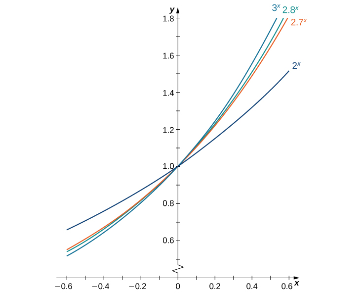
Figure 1 provides graphs of the functions $y=2^x, \, y=3^x, \, y=2.7^x$ , and $y=2.8^x$ . Observing the slopes of tangent lines at $x=0$ for these functions provides empirical evidence suggesting that $e$ is approximately between $2.7$ and $2.8$ . This observation is supported by the graph where the tangent line at $x=0$ for $y=e^x$ has a slope of $1$ , uniquely defining $e$ as approximately $2.718$ .

The graphs of 3x, 2.8x, 2.7x, and 2x are shown. In quadrant I, their order from least to greatest is 2x, 2.7x, 2.8x, and 3x. In quadrant II, this order is reversed. All cross the y-axis at (0, 1). — Figure 1. The graph of $E(x)=e^x$ is between $y=2^x$ and $y=3^x$ .

The natural exponential function, $E(x)=e^x$ , and its inverse, the natural logarithm $L(x)=\log_e x=\ln x$ are essential for understanding continuous growth and decay processes modeled in various scientific and financial contexts.

To estimate the value of $e$ , we consider the derivative of exponential functions of the form $B(x)=b^x$ at $x=0$ , denoted as $B^{\prime}(0)$ .

To accurately determine $B^{\prime}(0)$ , we select values of x very close to zero, such as $x=0.00001$ and $x=-0.00001$ . This method allows us to find $B^{\prime}(0)$ and compare it against our hypothesized value of $b$ that satisfies $B^{\prime}(0)=1$ , indicating $b=e$ .

The table below illustrates how varying $b$ around the theoretical value of $e$ allows us to pinpoint the exact value where $B^{\prime}(0) \approx 1$ , suggesting $e \approx 2.718$ .

Estimating a Value of $e$
$b$	$\frac{b^{-0.00001}-1}{-0.00001} < B^{\prime}(0) < \frac{b^{0.00001}-1}{0.00001}$	$b$	$\frac{b^{-0.00001}-1}{-0.00001} < B^{\prime}(0) < \frac{b^{0.00001}-1}{0.00001}$
$2$	$0.693145 < B^{\prime}(0) < 0.69315$	$2.7183$	$1.000002 < B^{\prime}(0) < 1.000012$
$2.7$	$0.993247 < B^{\prime}(0) < 0.993257$	$2.719$	$1.000259 < B^{\prime}(0) < 1.000269$
$2.71$	$0.996944 < B^{\prime}(0) < 0.996954$	$2.72$	$1.000627 < B^{\prime}(0) < 1.000637$
$2.718$	$0.999891 < B^{\prime}(0) < 0.999901$	$2.8$	$1.029614 < B^{\prime}(0) < 1.029625$
$2.7182$	$0.999965 < B^{\prime}(0) < 0.999975$	$3$	$1.098606 < B^{\prime}(0) < 1.098618$

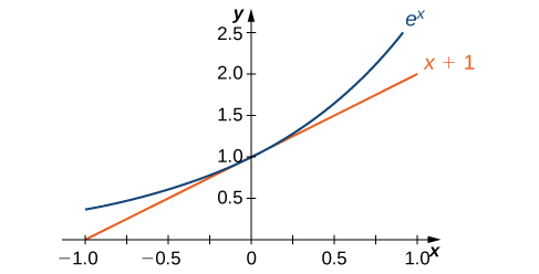
The graph of $E(x)=e^x$ is shown alongside the line $y=x+1$ in Figure 2, demonstrating that the tangent to $E(x)=e^x$ at $x=0$ has a slope of $1$ . This observation supports the hypothesis that the value of $e$ optimizes the slope at $x=0$ to exactly $1$ .

Graph of the function ex along with its tangent at (0, 1), x + 1. — Figure 2. The tangent line to $E(x)=e^x$ at $x=0$ has slope 1.

Now that we understand the underlying behavior at $x=0$ , let’s derive the general derivative formula for $B(x)=b^x, \, b>0$ . We start by applying the limit definition of the derivative:

B^{'} (0) = lim_{h \to 0} \frac{b^{0 + h} - b^{0}}{h} = lim_{h \to 0} \frac{b^{h} - 1}{h}

$B^{\prime}(0)=\underset{h\to 0}{\lim}\dfrac{b^{0+h}-b^0}{h}=\underset{h\to 0}{\lim}\dfrac{b^h-1}{h}$

Turning to $B^{\prime}(x)$ , we obtain the following.

\begin{array}{lllll} B^{'} (x) & = lim_{h \to 0} \frac{b^{x + h} - b^{x}}{h} & Apply the limit definition of the derivative. \\ = lim_{h \to 0} \frac{b^{x} b^{h} - b^{x}}{h} & Note that b^{x + h} = b^{x} b^{h} . \\ = lim_{h \to 0} \frac{b^{x} (b^{h} - 1)}{h} & Factor out b^{x} . \\ = b^{x} lim_{h \to 0} \frac{b^{h} - 1}{h} & Apply a property of limits. \\ = b^{x} B^{'} (0) & Use B^{'} (0) = lim_{h \to 0} \frac{b^{0 + h} - b^{0}}{h} = lim_{h \to 0} \frac{b^{h} - 1}{h} . \end{array}

$\begin{array}{lllll} B^{\prime}(x) & =\underset{h\to 0}{\lim}\frac{b^{x+h}-b^x}{h} & & & \text{Apply the limit definition of the derivative.} \\ & =\underset{h\to 0}{\lim}\frac{b^xb^h-b^x}{h} & & & \text{Note that} \, b^{x+h}=b^x b^h. \\ & =\underset{h\to 0}{\lim}\frac{b^x(b^h-1)}{h} & & & \text{Factor out} \, b^x. \\ & =b^x\underset{h\to 0}{\lim}\frac{b^h-1}{h} & & & \text{Apply a property of limits.} \\ & =b^x B^{\prime}(0) & & & \text{Use} \, B^{\prime}(0)=\underset{h\to 0}{\lim}\frac{b^{0+h}-b^0}{h}=\underset{h\to 0}{\lim}\frac{b^h-1}{h}. \end{array}$

We see that on the basis of the assumption that $B(x)=b^x$ is differentiable at $0, \, B(x)$ is not only differentiable everywhere, but its derivative is

B^{'} (x) = b^{x} B^{'} (0)

$B^{\prime}(x)=b^x B^{\prime}(0)$

For $E(x)=e^x, \, E^{\prime}(0)=1$ . Thus, we have $E^{\prime}(x)=e^x$ . (The value of $B^{\prime}(0)$ for an arbitrary function of the form $B(x)=b^x, \, b>0$ , will be derived later.)

derivative of the natural exponential function

Let $E(x)=e^x$ be the natural exponential function. Then

E^{'} (x) = e^{x}

$E^{\prime}(x)=e^x$

In general,

\frac{d}{d x} (e^{g (x)}) = e^{g (x)} g^{'} (x)

$\frac{d}{dx}(e^{g(x)})=e^{g(x)} g^{\prime}(x)$

If it helps, think of the formula as the chain rule being applied to natural exponential functions. The derivative of ${e}$ raised to the power of a function will simply be ${e}$ raised to the power of the function multiplied by the derivative of that function.

Find the derivative of $f(x)=e^{\tan (2x)}$ .

Using the derivative formula and the chain rule,

\begin{array}{ll} f^{'} (x) & = e^{\tan (2 x)} \frac{d}{d x} (\tan (2 x)) \\ = e^{\tan (2 x)} \sec^{2} (2 x) \cdot 2. \end{array}

$\begin{array}{ll} f^{\prime}(x) & =e^{\tan (2x)}\frac{d}{dx}(\tan (2x)) \\ & = e^{\tan (2x)} \sec^2 (2x) \cdot 2. \end{array}$

Find the derivative of $y=\dfrac{e^{x^2}}{x}$ .

Use the derivative of the natural exponential function, the quotient rule, and the chain rule.

\begin{array}{lllll} y^{'} & = \frac{(e^{x^{2}} \cdot 2 x) \cdot x - 1 \cdot e^{x^{2}}}{x^{2}} & Apply the quotient rule. \\ = \frac{e^{x^{2}} (2 x^{2} - 1)}{x^{2}} & Simplify. \end{array}

$\begin{array}{lllll} y^{\prime} & =\large \frac{(e^{x^2} \cdot 2x) \cdot x - 1 \cdot e^{x^2}}{x^2} & & & \text{Apply the quotient rule.} \\ & = \large \frac{e^{x^2}(2x^2-1)}{x^2} & & & \text{Simplify.} \end{array}$

A colony of mosquitoes has an initial population of $1000.$ After $t$ days, the population is given by $A(t)=1000e^{0.3t}$ . Show that the ratio of the rate of change of the population, $A^{\prime}(t)$ , to the population size, $A(t)$ is constant.

First find $A^{\prime}(t)$ . By using the chain rule, we have $A^{\prime}(t)=300e^{0.3t}$ . Thus, the ratio of the rate of change of the population to the population size is given by

\frac{A^{'} (t)}{A (t)} = \frac{300 e^{0.3 t}}{1000 e^{0.3 t}} = 0.3

$\large \frac{A^{\prime}(t)}{A(t)} \normalsize = \large \frac{300e^{0.3t}}{1000e^{0.3t}}=0.3$

The ratio of the rate of change of the population to the population size is the constant $0.3$ .

Watch the following video to see the worked solution to this example.

For closed captioning, open the video on its original page by clicking the Youtube logo in the lower right-hand corner of the video display. In YouTube, the video will begin at the same starting point as this clip, but will continue playing until the very end.

You can view the transcript for this segmented clip of “3.9 Derivatives of Exponential and Logarithmic Functions” here (opens in new window).