Derivatives as Rates of Change: Learn It 1

Lumen Learning

Derivatives as Rates of Change: Learn It 1

Calculate how quantities change on average over time
Use rates of change to figure out how an object’s position, speed, and acceleration are changing over time
Estimate future population sizes using current data and how fast the population is growing
Use derivatives to determine the cost and revenue of producing one more unit in a business

Amount of Change Formula

One application of derivatives is to estimate an unknown value of a function at a point by using a known value of the function at some given point together with its rate of change at that given point.

If $f(x)$ is a function defined on an interval $[a,a+h]$ , then the amount of change of $f(x)$ over the interval is the change in the $y$ values of the function over that interval and is given by:

f (a + h) - f (a)

$f(a+h)-f(a)$

The average rate of change of the function $f$ over that same interval is the ratio of the amount of change over that interval to the corresponding change in the $x$ values. It is given by:

\frac{f (a + h) - f (a)}{h}

$\dfrac{f(a+h)-f(a)}{h}$

As we already know, the instantaneous rate of change of $f(x)$ at $a$ is its derivative,

f^{'} (a) = lim_{h \to 0} \frac{f (a + h) - f (a)}{h}

$f^{\prime}(a)=\underset{h\to 0}{\lim}\dfrac{f(a+h)-f(a)}{h}$

For small enough values of $h, \, f^{\prime}(a)\approx \frac{f(a+h)-f(a)}{h}$ . We can then solve for $f(a+h)$ to get the amount of change formula:

f (a + h) \approx f (a) + f^{'} (a) h

$f(a+h)\approx f(a)+f^{\prime}(a)h$

We can use this formula if we know only $f(a)$ and $f^{\prime}(a)$ and wish to estimate the value of $f(a+h)$ . For example, we may use the current population of a city and the rate at which it is growing to estimate its population in the near future.

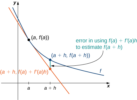
As we can see in Figure 1, we are approximating $f(a+h)$ by the $y$ coordinate at $a+h$ on the line tangent to $f(x)$ at $x=a$ . Observe that the accuracy of this estimate depends on the value of $h$ as well as the value of $f^{\prime}(a)$ .

On the Cartesian coordinate plane with a and a + h marked on the x axis, the function f is graphed. It passes through (a, f(a)) and (a + h, f(a + h)). A straight line is drawn through (a, f(a)) with its slope being the derivative at that point. This straight line passes through (a + h, f(a) + f’(a)h). There is a line segment connecting (a + h, f(a + h)) and (a + h, f(a) + f’(a)h), and it is marked that this is the error in using f(a) + f’(a)h to estimate f(a + h). — Figure 1. The new value of a changed quantity equals the original value plus the rate of change times the interval of change: $f(a+h)\approx f(a)+f^{\prime}(a)h$ .

average rate of change

The average rate of change of a function $f$ over the interval $[a,a+h]$ is the ratio of the amount of change in $f$ over that interval to the corresponding change in $x$ values.

The average rate of change is given by:

\frac{f (a + h) - f (a)}{h}

$\dfrac{f(a+h)-f(a)}{h}$

Here is an interesting demonstration of rate of change.

If $f(3)=2$ and $f^{\prime}(3)=5$ , estimate $f(3.2)$ .

Begin by finding $h$ . We have $h=3.2-3=0.2$ . Thus,

f (3.2) = f (3 + 0.2) \approx f (3) + (0.2) f^{'} (3) = 2 + 0.2 (5) = 3

$f(3.2)=f(3+0.2)\approx f(3)+(0.2)f^{\prime}(3)=2+0.2(5)=3$ .

Watch the following video to see the worked solution to this example.

For closed captioning, open the video on its original page by clicking the Youtube logo in the lower right-hand corner of the video display. In YouTube, the video will begin at the same starting point as this clip, but will continue playing until the very end.

You can view the transcript for this segmented clip of “3.4 Derivatives as Rates of Change” here (opens in new window).