The first derivative test provides a systematic approach to identify local extrema, but in some cases, using the second derivative can be more straightforward. A function must have a local extremum at a critical point, but not all critical points are extremas.
Consider a function [latex]f[/latex] that is twice-differentiable on an open interval [latex]I[/latex] containing [latex]a[/latex].
If [latex]f^{\prime \prime}(x)<0[/latex] and [latex]f^{\prime}(a)=0[/latex], [latex]f[/latex]is concave down at [latex]a[/latex], indicating a local maximum.
If [latex]f^{\prime \prime}(x)>0[/latex] and [latex]f^{\prime}(a)=0[/latex], [latex]f[/latex]is concave up at [latex]a[/latex], suggesting a local minimum at [latex]a[/latex].
Furthermore, if [latex]f^{\prime \prime}[/latex] is continuous over [latex]I[/latex] and remains positive, [latex]f[/latex] is consistently concave up across [latex]I[/latex], which helps in determining the behavior of [latex]f[/latex] at other critical points.
For instance, suppose there exists a point [latex]b[/latex] such that [latex]f^{\prime}(b)=0[/latex] and [latex]f^{\prime \prime}[/latex] is positive throughout, [latex]f[/latex] has a local minimum at [latex]b[/latex]. The second derivative thus confirms the nature of local extrema by providing insight into the concavity of the function at critical points.
Figure 9. Consider a twice-differentiable function [latex]f[/latex] such that [latex]f^{\prime \prime}[/latex] is continuous. Since [latex]f^{\prime}(a)=0[/latex] and [latex]f^{\prime \prime}(a)<0[/latex], there is an interval [latex]I[/latex] containing [latex]a[/latex] such that for all [latex]x[/latex] in [latex]I[/latex], [latex]f[/latex] is increasing if [latex]x<a[/latex] and [latex]f[/latex] is decreasing if [latex]x>a[/latex]. As a result, [latex]f[/latex] has a local maximum at [latex]x=a[/latex]. Since [latex]f^{\prime}(b)=0[/latex] and [latex]f^{\prime \prime}(b)>0[/latex], there is an interval [latex]I[/latex] containing [latex]b[/latex] such that for all [latex]x[/latex] in [latex]I[/latex], [latex]f[/latex] is decreasing if [latex]x<b[/latex] and [latex]f[/latex] is increasing if [latex]x>b[/latex]. As a result, [latex]f[/latex] has a local minimum at [latex]x=b[/latex].
second derivative test
Suppose [latex]f^{\prime}(c)=0, \, f^{\prime \prime}[/latex] is continuous over an interval containing [latex]c[/latex].
If [latex]f^{\prime \prime}(c)>0[/latex], then [latex]f[/latex] has a local minimum at [latex]c[/latex].
If [latex]f^{\prime \prime}(c)<0[/latex], then [latex]f[/latex] has a local maximum at [latex]c[/latex].
If [latex]f^{\prime \prime}(c)=0[/latex], then the test is inconclusive.
Note that for case iii. when [latex]f^{\prime \prime}(c)=0[/latex], then [latex]f[/latex] may have a local maximum, local minimum, or neither at [latex]c[/latex].
The functions [latex]f(x)=x^3[/latex], [latex]f(x)=x^4[/latex], and [latex]f(x)=−x^4[/latex] all have critical points at [latex]x=0[/latex]. In each case, the second derivative is zero at [latex]x=0[/latex].
However, the function [latex]f(x)=x^4[/latex] has a local minimum at [latex]x=0[/latex] whereas the function [latex]f(x)=−x^4[/latex] has a local maximum at [latex]x=0[/latex] and the function [latex]f(x)=x^3[/latex] does not have a local extremum at [latex]x=0[/latex].
Let’s now look at how to use the second derivative test to determine whether [latex]f[/latex] has a local maximum or local minimum at a critical point [latex]c[/latex] where [latex]f^{\prime}(c)=0[/latex].
Use the second derivative to find the location of all local extrema for [latex]f(x)=x^5-5x^3[/latex].
To apply the second derivative test, we first need to find critical points [latex]c[/latex] where [latex]f^{\prime}(c)=0[/latex].
The derivative is [latex]f^{\prime}(x)=5x^4-15x^2[/latex]. Therefore, [latex]f^{\prime}(x)=5x^4-15x^2=5x^2(x^2-3)=0[/latex] when [latex]x=0,\pm \sqrt{3}[/latex].
To determine whether [latex]f[/latex] has a local extrema at any of these points, we need to evaluate the sign of [latex]f^{\prime \prime}[/latex] at these points. The second derivative is
In the following table, we evaluate the second derivative at each of the critical points and use the second derivative test to determine whether [latex]f[/latex] has a local maximum or local minimum at any of these points.
[latex]x[/latex]
[latex]f^{\prime \prime}(x)[/latex]
Conclusion
[latex]−\sqrt{3}[/latex]
[latex]-30\sqrt{3}[/latex]
Local maximum
[latex]0[/latex]
[latex]0[/latex]
Second derivative test is inconclusive
[latex]\sqrt{3}[/latex]
[latex]30\sqrt{3}[/latex]
Local minimum
By the second derivative test, we conclude that [latex]f[/latex] has a local maximum at [latex]x=−\sqrt{3}[/latex] and [latex]f[/latex] has a local minimum at [latex]x=\sqrt{3}[/latex]. The second derivative test is inconclusive at [latex]x=0[/latex].
To determine whether [latex]f[/latex] has a local extrema at [latex]x=0[/latex], we apply the first derivative test.
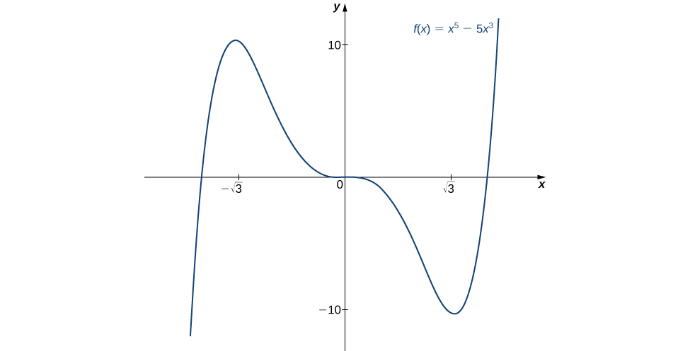
To evaluate the sign of [latex]f^{\prime}(x)=5x^2(x^2-3)[/latex] for [latex]x \in (−\sqrt{3},0)[/latex] and [latex]x \in (0,\sqrt{3})[/latex], let [latex]x=-1[/latex] and [latex]x=1[/latex] be the two test points. Since [latex]f^{\prime}(-1)<0[/latex] and [latex]f^{\prime}(1)<0[/latex], we conclude that [latex]f[/latex] is decreasing on both intervals and, therefore, [latex]f[/latex] does not have a local extrema at [latex]x=0[/latex] as shown in the following graph.
Figure 10. The function [latex]f[/latex] has a local maximum at [latex]x=−\sqrt{3}[/latex] and a local minimum at [latex]x=\sqrt{3}[/latex]
Watch the following video to see the worked solution to this example.
For closed captioning, open the video on its original page by clicking the Youtube logo in the lower right-hand corner of the video display. In YouTube, the video will begin at the same starting point as this clip, but will continue playing until the very end.