Derivatives and the Shape of a Graph: Learn It 1

Lumen Learning

Derivatives and the Shape of a Graph: Learn It 1

Use the first derivative to determine where a function is going up or down, and identify points that might be local highs or lows
Apply the second derivative to find out where a function curves upward or downward and locate points where this curvature changes
Use the second derivative test to determine if a point on a graph is the highest or lowest within specific sections

The First Derivative Test

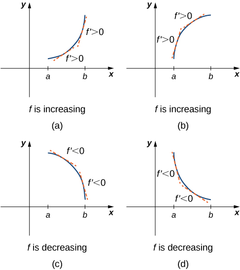
Corollary 3 of the Mean Value Theorem showed that if the derivative of a function is positive over an interval $I$ then the function is increasing over $I$ . On the other hand, if the derivative of the function is negative over an interval $I$ , then the function is decreasing over $I$ as shown in the following figure.

This figure is broken into four figures labeled a, b, c, and d. Figure a shows a function increasing convexly from (a, f(a)) to (b, f(b)). At two points the derivative is taken and it is noted that at both f’ > 0. In other words, f is increasing. Figure b shows a function increasing concavely from (a, f(a)) to (b, f(b)). At two points the derivative is taken and it is noted that at both f’ > 0. In other words, f is increasing. Figure c shows a function decreasing concavely from (a, f(a)) to (b, f(b)). At two points the derivative is taken and it is noted that at both f’ < 0. In other words, f is decreasing. Figure d shows a function decreasing convexly from (a, f(a)) to (b, f(b)). At two points the derivative is taken and it is noted that at both f’ < 0. In other words, f is decreasing. — Figure 1. Both functions are increasing over the interval $(a,b)$ . At each point $x$ , the derivative $f^{\prime}(x)>0$ . Both functions are decreasing over the interval $(a,b)$ . At each point $x$ , the derivative $f^{\prime}(x)<0$ .

A continuous function $f$ has a local maximum at point $c$ if and only if $f$ switches from increasing to decreasing at point $c$ . Similarly, $f$ has a local minimum at $c$ if and only if $f$ switches from decreasing to increasing at $c$ .

If $f$ is a continuous function over an interval $I$ containing $c$ and differentiable over $I$ , except possibly at $c$ , the only way $f$ can switch from increasing to decreasing (or vice versa) at point $c$ is if ${f}^{\prime }$ changes sign as $x$ increases through $c.$

If $f$ is differentiable at $c,$ the only way that ${f}^{\prime }.$ can change sign as $x$ increases through $c$ is if $f^{\prime}(c)=0$ .

Therefore, for a function $f$ that is continuous over an interval $I$ containing $c$ and differentiable over $I$ , except possibly at $c$ , the only way $f$ can switch from increasing to decreasing (or vice versa) is if $f^{\prime}(c)=0$ or $f^{\prime}(c)$ is undefined.

Consequently, to locate local extrema for a function $f$ , we look for points $c$ in the domain of $f$ such that $f^{\prime}(c)=0$ or $f^{\prime}(c)$ is undefined. Recall that such points are called critical points of $f$ . Note that $f$ need not have a local extrema at a critical point. The critical points are candidates for local extrema only.

In Figure 2, we show that if a continuous function $f$ has a local extremum, it must occur at a critical point, but a function may not have a local extremum at a critical point. We show that if $f$ has a local extremum at a critical point, then the sign of $f^{\prime}$ switches as $x$ increases through that point.

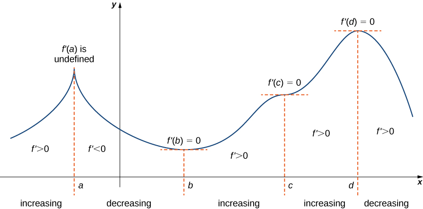
A function f(x) is graphed. It starts in the second quadrant and increases to x = a, which is too sharp and hence f’(a) is undefined. In this section f’ > 0. Then, f decreases from x = a to x = b (so f’ < 0 here), before increasing at x = b. It is noted that f’(b) = 0. While increasing from x = b to x = c, f’ > 0. The function has an inversion point at c, and it is marked f’(c) = 0. The function increases some more to d (so f’ > 0), which is the global maximum. It is marked that f’(d) = 0. Then the function decreases and it is marked that f’ > 0. — Figure 2. The function $f$ has four critical points: $a,b,c$ , and $d$ . The function $f$ has local maxima at $a$ and $d$ , and a local minimum at $b$ . The function $f$ does not have a local extremum at $c$ . The sign of $f^{\prime}$ changes at all local extrema.

Using Figure 2, we summarize the main results regarding local extrema.

If a continuous function $f$ has a local extremum, it must occur at a critical point $c$ .
The function has a local extremum at the critical point $c$ if and only if the derivative $f^{\prime}$ switches sign as $x$ increases through $c$ .
Therefore, to test whether a function has a local extremum at a critical point $c$ , we must determine the sign of $f^{\prime}(x)$ to the left and right of $c$ .

This result is known as the first derivative test.

first derivative test

Suppose that $f$ is a continuous function over an interval $I$ containing a critical point $c$ . If $f$ is differentiable over $I$ , except possibly at point $c$ , then $f(c)$ satisfies one of the following descriptions:

If $f^{\prime}$ changes sign from positive when $x < c$ to negative when $x > c$ , then $f(c)$ is a local maximum of $f$ .
If $f^{\prime}$ changes sign from negative when $x < c$ to positive when $x >$ , then $f(c)$ is a local minimum of $f$ .
If $f^{\prime}$ has the same sign for $x < c$ and $x>c$ , then $f(c)$ is neither a local maximum nor a local minimum of $f$ .

We can summarize the first derivative test as a strategy for locating local extrema.

How to: Use the First Derivative Test

To determine local extrema of a function $f(x)$ that is continuous on an interval $[a,b]$ , follow these steps:

1. Identify Critical Points: Find all critical points of $f(x)$ within the interval and note these points along with the endpoints $a$ and $b$ .
2. Divide the Interval: Segment the interval $[a,b]$ using the critical points as boundaries, creating smaller subintervals.
3. Analyze the Sign of $f′(x)$ : Evaluate the derivative $f' (x)$ within each subinterval. A change in the sign of $f' (x)$ across a critical point indicates a local extremum at that point:
  - If $f′(x)$ changes from positive to negative, $f(x)$ has a local maximum at the critical point.
  - If $f′(x)$ changes from negative to positive, $f(x)$ has a local minimum at the critical point.
  - If $f′(x)$ does not change sign, $f(x)$ does not have a local extremum at that critical point.
4. Compare Values: Evaluate $f(x)$ at the critical points and endpoints to identify the absolute maximum and minimum over the interval.

Recall that when talking about local extrema, the value of the extremum is the $y$ value and the location of the extremum is the $x$ value.

Now let’s look at how to use this strategy to locate all local extrema for particular functions.

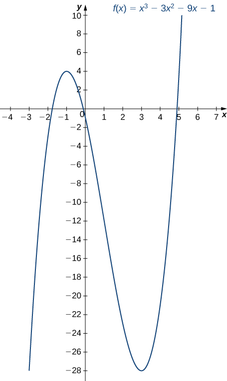
Use the first derivative test to find the location of all local extrema for $f(x)=x^3-3x^2-9x-1$ . Use a graphing utility to confirm your results.

Step 1. The derivative is $f^{\prime}(x)=3x^2-6x-9$ . To find the critical points, we need to find where $f^{\prime}(x)=0$ . Factoring the polynomial, we conclude that the critical points must satisfy:

3 (x^{2} - 2 x - 3) = 3 (x - 3) (x + 1) = 0

$3(x^2-2x-3)=3(x-3)(x+1)=0$

Therefore, the critical points are $x=3,-1$ . Now divide the interval $(−\infty ,\infty)$ into the smaller intervals $(−\infty ,-1), \, (-1,3)$ , and $(3,\infty)$ .

Step 2. Since $f^{\prime}$ is a continuous function, to determine the sign of $f^{\prime}(x)$ over each subinterval, it suffices to choose a point over each of the intervals $(−\infty ,-1), \, (-1,3)$ , and $(3,\infty)$ and determine the sign of $f^{\prime}$ at each of these points.

For example, let’s choose $x=-2, \, x=0$ , and $x=4$ as test points.

Interval	Test Point	Sign of $f^{\prime}(x)=3(x-3)(x+1)$ at Test Point	Conclusion
$(−\infty ,-1)$	$x=-2$	$(+)(−)(−)=+$	$f$ is increasing.
$(-1,3)$	$x=0$	$(+)(−)(+)=−$	$f$ is decreasing.
$(3,\infty)$	$x=4$	$(+)(+)(+)=+$	$f$ is increasing.

Step 3. Since $f^{\prime}$ switches sign from positive to negative as $x$ increases through $1, \, f$ has a local maximum at $x=-1$ .

Since $f^{\prime}$ switches sign from negative to positive as $x$ increases through $3, \, f$ has a local minimum at $x=3$ .

These analytical results agree with the following graph.

The function f(x) = x3 – 3x2 – 9x – 1 is graphed. It has a maximum at x = −1 and a minimum at x = 3. The function is increasing before x = −1, decreasing until x = 3, and then increasing after that. — Figure 3. The function $f$ has a maximum at $x=-1$ and a minimum at $x=3$

Watch the following video to see the worked solution to this example.

For closed captioning, open the video on its original page by clicking the Youtube logo in the lower right-hand corner of the video display. In YouTube, the video will begin at the same starting point as this clip, but will continue playing until the very end.

You can view the transcript for this segmented clip of “4.5 Derivatives and the Shape of a Graph” here (opens in new window).

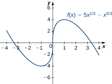
Use the first derivative test to find the location of all local extrema for $f(x)=5x^{\frac{1}{3}}-x^{\frac{5}{3}}$ . Use a graphing utility to confirm your results.

Step 1. The derivative is

f^{'} (x) = \frac{5}{3} x^{- 2 / 3} - \frac{5}{3} x^{2 / 3} = \frac{5}{3 x^{2 / 3}} - \frac{5 x^{2 / 3}}{3} = \frac{5 - 5 x^{4 / 3}}{3 x^{2 / 3}} = \frac{5 (1 - x^{4 / 3})}{3 x^{2 / 3}}

$f^{\prime}(x)=\frac{5}{3}x^{-2/3}-\frac{5}{3}x^{2/3}=\frac{5}{3x^{2/3}}-\frac{5x^{2/3}}{3}=\frac{5-5x^{4/3}}{3x^{2/3}}=\frac{5(1-x^{4/3})}{3x^{2/3}}$ .

The derivative $f^{\prime}(x)=0$ when $1-x^{4/3}=0$ . Therefore, $f^{\prime}(x)=0$ at $x=\pm 1$ .

The derivative $f^{\prime}(x)$ is undefined at $x=0$ . Therefore, we have three critical points: $x=0$ , $x=1$ , and $x=-1$ .

Consequently, divide the interval $(−\infty ,\infty)$ into the smaller intervals $(−\infty ,-1), \, (-1,0), \, (0,1)$ , and $(1,\infty )$ .

Step 2: Since $f^{\prime}$ is continuous over each subinterval, it suffices to choose a test point $x$ in each of the intervals from step 1 and determine the sign of $f^{\prime}$ at each of these points. The points $x=-2, \, x=-\frac{1}{2}, \, x=\frac{1}{2}$ , and $x=2$ are test points for these intervals.

Interval	Test Point	Sign of $f^{\prime}(x)=\frac{5(1-x^{4/3})}{3x^{2/3}}$ at Test Point	Conclusion
$(−\infty ,-1)$	$x=-2$	$\frac{(+)(−)}{+}=−$	$f$ is decreasing.
$(-1,0)$	$x=-\frac{1}{2}$	$\frac{(+)(+)}{+}=+$	$f$ is increasing.
$(0,1)$	$x=\frac{1}{2}$	$\frac{(+)(+)}{+}=+$	$f$ is increasing.
$(1,\infty )$	$x=2$	$\frac{(+)(−)}{+}=−$	$f$ is decreasing.

Step 3: Since $f$ is decreasing over the interval $(−\infty ,-1)$ and increasing over the interval $(-1,0)$ , $f$ has a local minimum at $x=-1$ .

Since $f$ is increasing over the interval $(-1,0)$ and the interval $(0,1)$ , $f$ does not have a local extremum at $x=0$ .

Since $f$ is increasing over the interval $(0,1)$ and decreasing over the interval $(1,\infty ), \, f$ has a local maximum at $x=1$ .

The analytical results agree with the following graph.

The function f(x) = 5x1/3 – x5/3 is graphed. It decreases to its local minimum at x = −1, increases to x = 1, and then decreases after that. — Figure 4. The function f has a local minimum at $x=-1$ and a local maximum at $x=1$ .