Velocities and Rates of Change
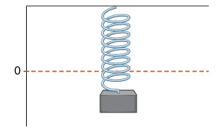
Now that we can evaluate a derivative, we can apply it to velocity problems. Recall that if [latex]s(t)[/latex] is the position of an object moving along a coordinate axis, the average velocity of the object over a time interval [latex][a,t][/latex] if [latex]t>a[/latex] or [latex][t,a][/latex] if [latex]t As the values of [latex]t[/latex] approach [latex]a[/latex], the values of [latex]v_{\text{avg}}[/latex] approach the value we call the instantaneous velocity at [latex]a[/latex]. That is, instantaneous velocity at [latex]a[/latex], denoted [latex]v(a)[/latex], is given by To better understand the relationship between average velocity and instantaneous velocity, see Figure 7. In this figure, the slope of the tangent line (shown in red) is the instantaneous velocity of the object at time [latex]t=a[/latex]. The slope of the secant line (shown in green) is the average velocity of the object over the time interval [latex][a,t][/latex]. We can use the definitions to calculate the instantaneous velocity, or we can estimate the velocity of a moving object by using a table of values. We can then confirm the estimate by using the difference quotient. A lead weight on a spring is oscillating up and down. Its position at time [latex]t[/latex] with respect to a fixed horizontal line is given by [latex]s(t)= \sin t[/latex]. Use a table of values to estimate [latex]v(0)[/latex]. Check the estimate by using the definition of a derivative. As we have seen throughout this section, the slope of a tangent line to a function and instantaneous velocity are related concepts. Each is calculated by computing a derivative and each measures the instantaneous rate of change of a function, or the rate of change of a function at any point along the function. The instantaneous rate of change of a function [latex]f(x)[/latex] at a value [latex]a[/latex] is its derivative [latex]f^{\prime}(a)[/latex]. A homeowner sets the thermostat so that the temperature in the house begins to drop from [latex]70^{\circ}\text{F}[/latex] at 9 p.m., reaches a low of [latex]60^{\circ}[/latex] during the night, and rises back to [latex]70^{\circ}[/latex] by 7 a.m. the next morning. Suppose that the temperature in the house is given by [latex]T(t)=0.4t^2-4t+70[/latex] for [latex]0\le t\le 10[/latex], where [latex]t[/latex] is the number of hours past 9 p.m. Find the instantaneous rate of change of the temperature at midnight.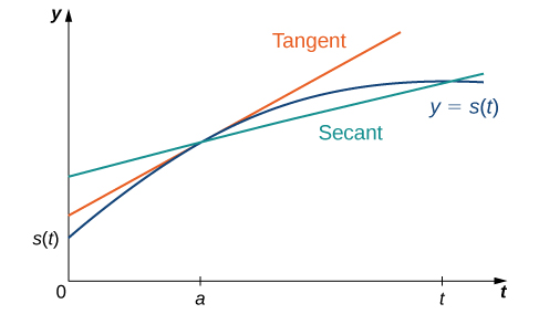
instantaneous rate of change